
SSA: Wigglez Spectra enhanced by the Data Central API
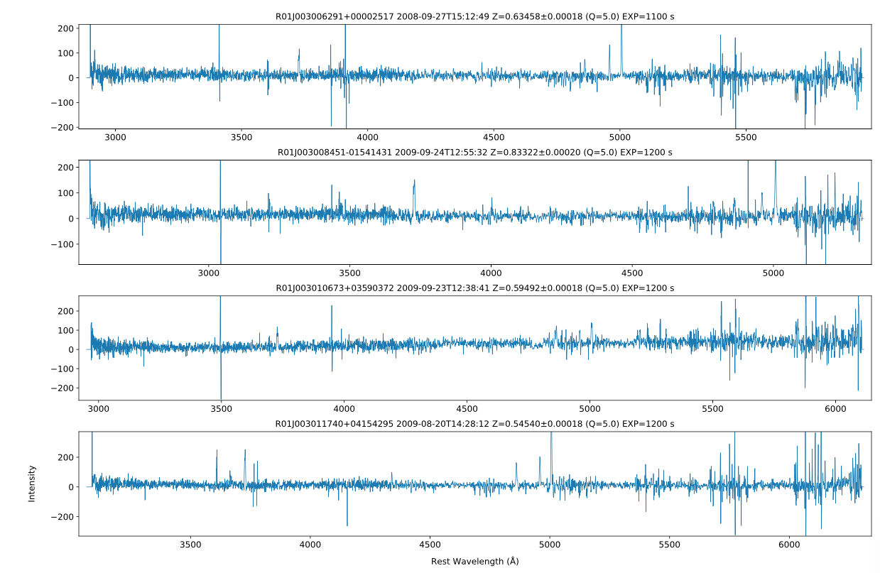
Example output of the example script to access Wigglez spectra. Note the redshift quality flag Q is obtained by the query to the DataCentral API.
In this example we use the Data Central API to select Wigglez spectra with a high redshift quality (Q) and then retrieve the spectra using the SSA service.
from specutils import Spectrum1D
import matplotlib.pyplot as plt
import matplotlib as mpl
from matplotlib.backends.backend_pdf import PdfPages
from matplotlib import gridspec
import numpy as np
import pandas as pd
from matplotlib import gridspec
from astropy.stats import sigma_clip
from astropy.time import Time
import requests
from io import BytesIO
from pyvo.dal.ssa  import search, SSAService

#set the figure size to be wide in the horizontal direction
#to accommodate the image cutouts alongside the spectra
fsize=[20,13]
mpl.rcParams['axes.linewidth'] = 0.7
FSIZE=12
LWIDTH=0.5
LABELSIZE=10

#Query the DataCentral API
#see https://datacentral.org.au/services/schema/#wigglez.final.catalogues.WiggleZData for more details
sql_query = "SELECT TOP 8 WiggleZ_Name,redshift,Dredshift,Q FROM wigglez_final.WiggleZCat WHERE Q = 5 and redshift BETWEEN 0.5 and 0.9"
api_url = 'https://datacentral.org.au/api/services/query/'
qdata = {'title' : 'wigglez_test_query',
         'notes' : 'test query for ssa example',
         'sql' : sql_query,
         'run_async' : False,
         'email'  : 'brent.miszalski@mq.edu.au'}
post = requests.post(api_url,data=qdata).json()
resp = requests.get(post['url']).json()
df = pd.DataFrame(resp['result']['data'],columns=resp['result']['columns'])
print (df)
#convert columns to floats - needed since data coming from json results
convertme = ['redshift','Dredshift','Q']
for c in convertme:
    df[c] = df[c].astype(float)
#put API results into a more accessible format
targets = np.array(df['WiggleZ_Name'])
redshift = np.array(df['redshift'])
redshift_err = np.array(df['Dredshift'])
Q = np.array(df['Q'])

#URL for DataCentral SSA service
url = "https://datacentral.org.au/vo/ssa/query"
service = SSAService(url)

#since SSA does not support more than one value per each parameter
#to query multiple targets we perform separate queries
#and append the results to indiv_results in the form of pandas dataframes
#Once done, we can concatenate the results into a single dataframe
#that makes processing the results a lot easier
#Note that we exclude the pos parameter here, since we are using the targetname

indiv_results = []
for idx in range(0,len(targets)):
    custom = {}
    custom['TARGETNAME'] = targets[idx]
    custom['COLLECTION'] = 'wigglez_final'
    results = service.search(**custom)
    indiv_results.append(results.votable.get_first_table().to_table(use_names_over_ids=True).to_pandas())

#dataframe containing all our results
df = pd.concat(indiv_results,ignore_index=True)

plotidx = 0
PLOT=1
pdf = PdfPages('wigglez.pdf')

#Number of spectra to plot
NSPEC = df.shape[0]
nrows = 4
ncolumns = 1

while plotidx < NSPEC:
    remaining = NSPEC - plotidx
    #setup a new plot for each grid of nrows by ncolumns spectra
    f = plt.figure(figsize=fsize)
    #We use gridspec to lay out the expected number of elements
    wr = [0.6]
    for w in range(0,ncolumns-1):
        wr.append(0.1)
    gs = gridspec.GridSpec(nrows,ncolumns,width_ratios=wr)
    gs.update(wspace=0.1,hspace=0.3)

    idx=0
    jdx=0

    running = 0
    for idx in range(0,nrows):
        for jdx in range(0,ncolumns):
            if(running == remaining):
                break
            if(jdx == 0):
                #need to add RESPONSEFORMAT=fits here to get fits format returned
                url= df.loc[plotidx,'access_url'] + "&RESPONSEFORMAT=fits"
                print ("Downloading ",url)
                #download and load the spectra using specutils Spectrum1D
                spec = Spectrum1D.read(BytesIO(requests.get(url).content),format='wcs1d-fits')
                z = df.loc[plotidx,'redshift']
                exptime = df.loc[plotidx,'t_exptime']

                ax = plt.subplot(gs[idx,jdx])
                ax.tick_params(axis='both', which='major', labelsize=FSIZE)
                ax.tick_params(axis='both', which='minor', labelsize=FSIZE)
                if(jdx == 0 and (idx == nrows-1 or idx == NSPEC-1)):
                   ax.set_xlabel("Rest Wavelength ($\mathrm{\AA}$)",labelpad=10, fontsize=FSIZE)
                   ax.set_ylabel("Intensity",labelpad=20, fontsize=FSIZE)
                #plot the spectrum
                ax.plot(spec.wavelength/(1+z),spec.flux,linewidth=LWIDTH)
                #now work out the best y-axis range to plot
                #use sigma clipping to determine the limits, but exclude 1 per cent of the wavelength range
                #at each end of the spectrum (often affected by noise or other systematic effects)
                nspec = len(spec.spectral_axis)
                clipped = sigma_clip(spec[int(0+0.01*nspec):int(nspec-0.01*nspec)].flux,masked=False,sigma=10)
                ymin = min(clipped).value
                ymax = max(clipped).value
                #print ("ymin/ymax: ",ymin,ymax)
                #xlims = ax.get_xlim()
                xmin = spec.wavelength[0].value/(1+z)
                xmax = spec.wavelength[nspec-1].value/(1+z)
                #add a 1% buffer either side of the x-range
                dx=0.01*(xmax-xmin)
                ax.set_xlim(xmin-dx,xmax+dx)
                #add a 1% buffer either side of the y-range
                dy=0.01*(ymax-ymin)
                ax.set_ylim(ymin-dy,ymax+dy)
                #make a nice title for each plot
                target = "%s" % df.loc[plotidx,'target_name']
                tmid = Time(df.loc[plotidx,'t_midpoint'],format='mjd')
                tmid.format='isot'
                red = "%.5f$\pm$%.5f" % (redshift[plotidx],redshift_err[plotidx])
                titre = "%s %s Z=%s (Q=%s) EXP=%d s" % (target,tmid.value[:-4],red,Q[plotidx],int(exptime))
                ax.set_title(titre)

                plotidx = plotidx + 1


                running=running + 1
    pdf.savefig()
    #plt.show()
    plt.close()
    PLOT=PLOT+1

pdf.close()