HiPS+MOC: Image cutouts with coverage checking and radio overlays
Background
In this example we extend the HiPS image cutout with radio overlay example by:
- Adding more optical survey HiPS data
- Checking for coverage using Multi-Order Coverage (MOC) maps
- Plotting all the data that we find has coverage for each target
These MOC maps are available for each of the HiPS datasets and can allow for a variety of neat applications.
That is, you can think of a MOC as a spatial outline of each HiPS dataset.
At the simplest level, it is very useful check if a target has spatial coverage by one of the surveys by using the MOCPy Python module. In order to run this example, you will need to install this module.
Additional documentation for the module can be found here.
Various complex operations can be performed on MOC maps (union, intersection, etc).
Creating a single MOC that is the intersection of several MOC maps may be useful to quickly check if a target has coverage in those surveys.
About this example
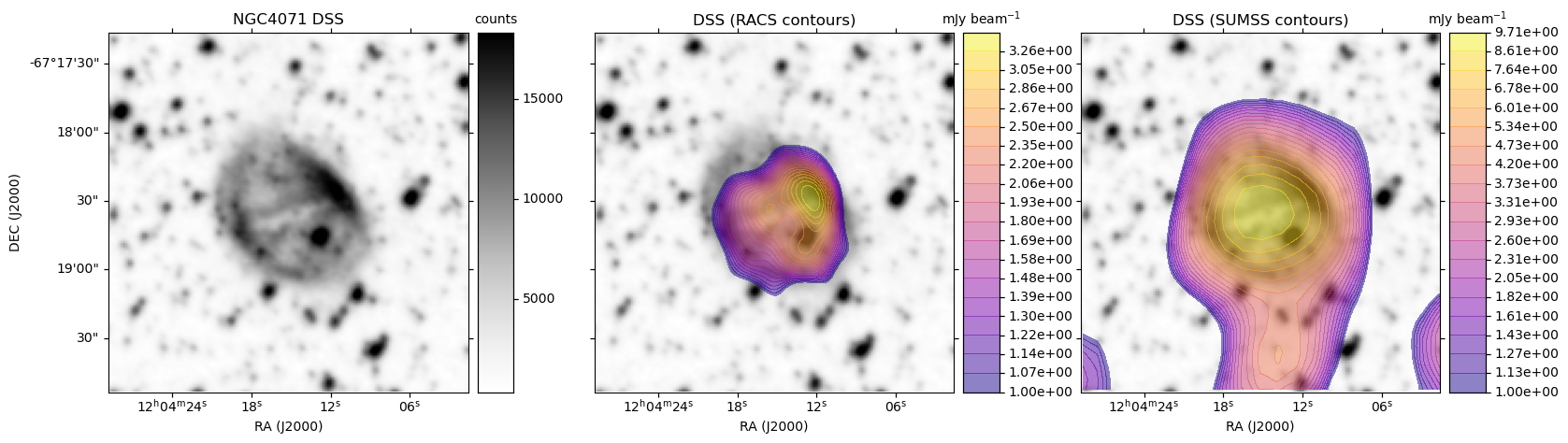
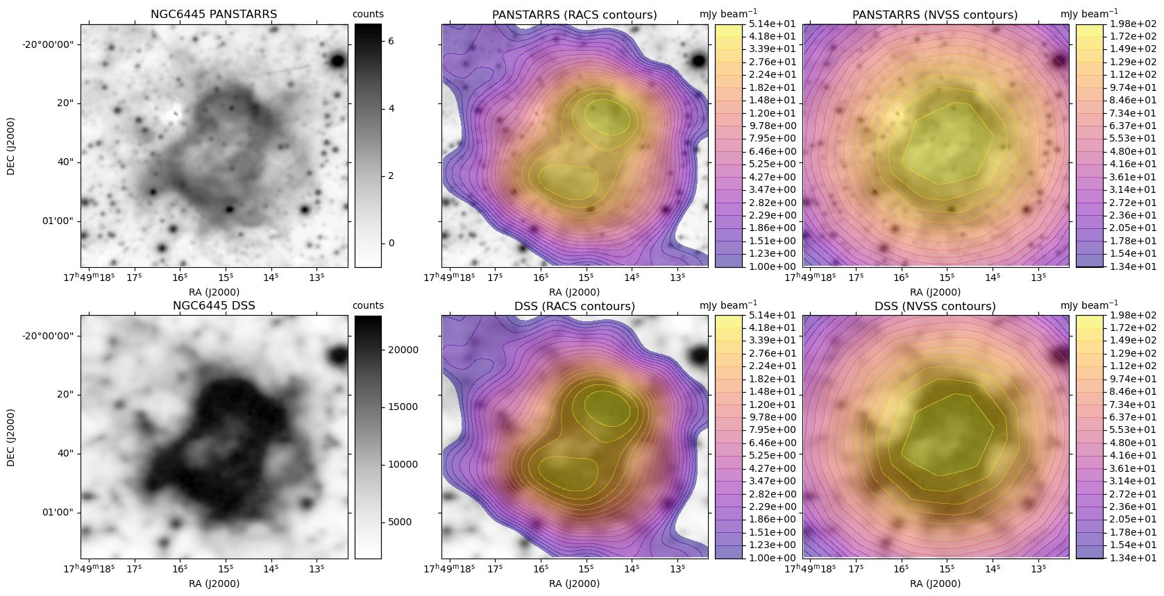
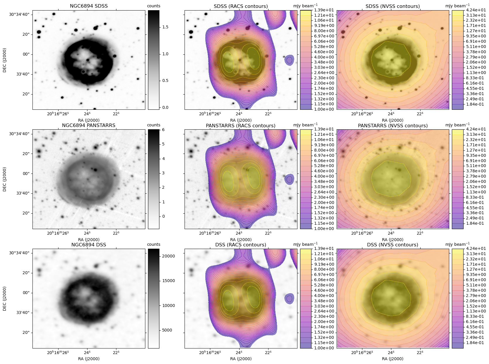
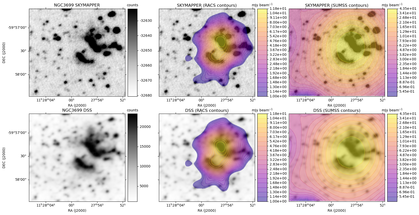
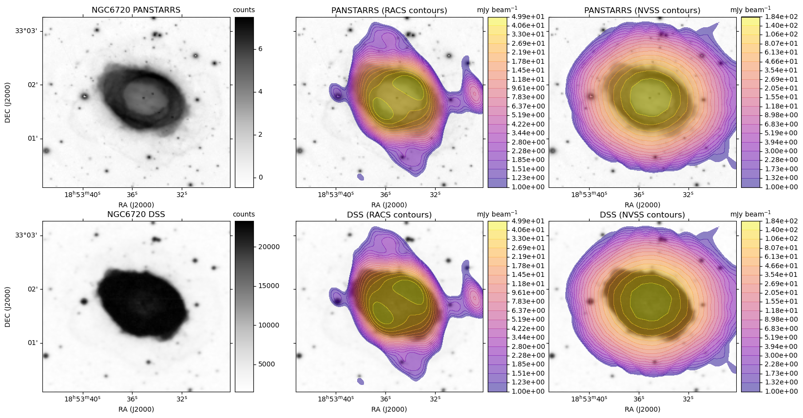
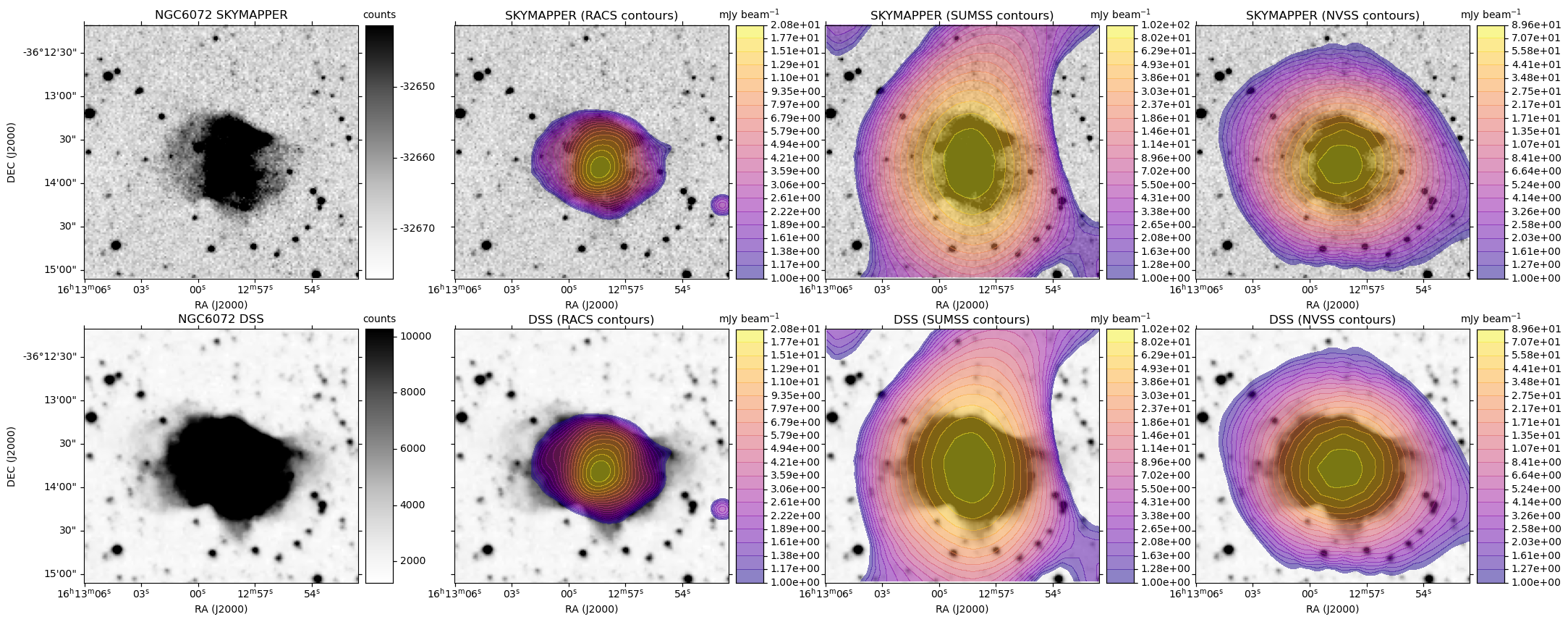
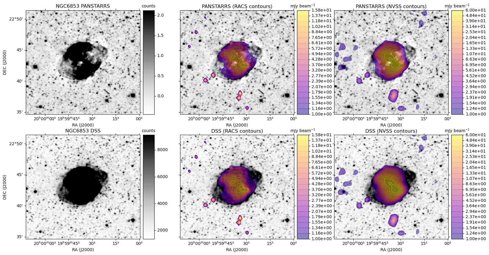
This example uses the Acker (Strasbourg-ESO) Catalogue of Galactic Planetary Nebulae to obtain positions to Planetary Nebulae (PNe) with optical diameters more than 30 arcsec. Samples of PNe that are part of the NGC catalogue are extracted separately for Northern and Southern positions based on their Declination.
For each sample we check whether the target positions have coverage in various MOC maps from the associated HiPS surveys.
This includes some R-band optical surveys and radio surveys.
If we find the MOC does not contain the target position, we do not request an image cutout from the corresponding survey data.
A plot is generated, similar to the HiPS image cutout with radio overlay example plots, except here each row is based on a single optical image. For each radio survey with coverage, the optical image is shown again with the radio contour overlay.
An important note about the HiPS data: In this example we have used HiPS data available from https://aladin.u-strasbg.fr/hips/list. These may not necessarily be the latest survey data available. For example, you can access images from more recent data releases of SkyMapper and PanSTARRS from elsewhere.
This example forms part of a series of General Virtual Observatory Examples developed by Data Central.
import matplotlib.pyplot as plt
import matplotlib as mpl
import numpy as np
import pandas as pd
from astropy.io import fits
from astropy.wcs import WCS
import re
from mpl_toolkits.axes_grid1 import make_axes_locatable
from urllib.parse import quote
import requests
from io import BytesIO
from mocpy import MOC
from astropy.visualization import ImageNormalize, MinMaxInterval, AsinhStretch,ZScaleInterval
from astropy import units as u
from astropy.io.votable import parse_single_table
import warnings
warnings.filterwarnings('ignore', category=UserWarning, append=True)

#urls to retrieve V/84 (Acker catalogue of PNe)
#Main table - object name and general info of PNe
umain = 'https://vizier.unistra.fr/viz-bin/votable?-source=V/84/main&-out.add=_RAJ2000%20_DEJ2000'
#Diameter table - optical and radio diameters of PNe
#filter: only those objects with optical diameters 30 arcsec or larger
udiam = 'https://vizier.unistra.fr/viz-bin/votable?-source=V/84/diam&oDiam=>30'

#urls of each HiPS survey (see https://aladin.u-strasbg.fr/hips/list for a larger list)
ohips = {
    'sdss' : 'http://alasky.u-strasbg.fr/SDSS/DR9/band-r/',
    'panstarrs' : 'http://alasky.u-strasbg.fr/Pan-STARRS/DR1/r/',
    'skymapper' : 'http://alasky.u-strasbg.fr/Skymapper/skymapper_R/',
    'dss' : 'http://alasky.u-strasbg.fr/DSS/DSS2Merged/',
}
rhips = {
    'racs' : 'https://www.atnf.csiro.au/research/RACS/RACS_I1/',
    'sumss' : 'http://alasky.u-strasbg.fr/SUMSS/',
    'nvss' : 'http://alasky.u-strasbg.fr/NVSS/intensity/',
}
#A function to make it easier to create a colorbar
#Adapted from https://joseph-long.com/writing/colorbars/
def colorbar(mappable,xlabel):
    last_axes = plt.gca()
    ax = mappable.axes
    fig = ax.figure
    divider = make_axes_locatable(ax)
    cax = divider.append_axes("right", size="10%", pad=0.1)
    #taking this approach to make a colorbar means the new axis is also of wcsaxes type
    #https://docs.astropy.org/en/stable/visualization/wcsaxes/
    #the following fixes up some issues and formats the colorbar
    cax.grid(False)
    cbar = fig.colorbar(mappable, cax=cax)
    cbar.ax.coords[1].set_ticklabel_position('r')
    cbar.ax.coords[1].set_auto_axislabel(False)
    cbar.ax.coords[0].set_ticks_visible(False)
    cbar.ax.coords[0].set_ticklabel_visible(False)
    cbar.ax.coords[1].set_axislabel(xlabel)
    cbar.ax.coords[1].set_axislabel_position('t')
    cbar.ax.coords[1].set_ticks_position('r')
    if(hasattr(mappable,'levels')):
        cbar.ax.coords[1].set_ticks(mappable.levels*u.dimensionless_unscaled)
        cbar.ax.coords[1].set_major_formatter('%.2e')
        #cbar.ax.coords[1].set_major_formatter('%.2f')
        cbar.ax.coords[1].set_ticklabel(exclude_overlapping=True)
    plt.sca(last_axes)
    return cbar


#A function to access the hips2fits service
#if the image is not empty, return the fits hdu
def get_hips_data(hips,pix_width, pix_height, diam, qra, qdec):
    url = 'http://alasky.u-strasbg.fr/hips-image-services/hips2fits?hips={}&width={}&height={}&fov={}&projection=TAN&coordsys=icrs&ra={}&dec={}&rotation_angle=0.0&format=fits'.format(quote(hips), pix_width, pix_height, diam*1.0/3600, qra, qdec)
    resp = requests.get(url)
    if(resp.status_code < 400):
        hdu = fits.open(BytesIO(resp.content))
        im = hdu[0].data
        if (not np.isnan(im[0][0])):
            return hdu
    else:
        return None
#A function to make each of the individual plots
#cnum = number of filled contour levels
#calpha = transparency of filled contours
def add_plot(ax,img,cimg,imlabel,clabel,pos,cnum = 20,calpha=0.5):
    #depending on where the image lies in the sequence (left, middle or right)
    #format the axes appropriately
    if(pos == 'l'):
        ax.coords[0].set_axislabel('RA (J2000)')
        ax.coords[1].set_axislabel('DEC (J2000)')

    if(pos == 'r'):
        ax.coords[1].set_ticklabel_position('r')
        ax.coords[1].set_axislabel_position('r')
        ax.coords[0].set_axislabel('RA (J2000)')
        ax.coords[1].set_axislabel('')
        ax.coords[1].set_auto_axislabel(False)
        ax.coords[1].set_ticklabel_visible(False)

    if(pos == 'm'):
         ax.coords[1].set_axislabel('')
         ax.coords[1].set_auto_axislabel(False)
         ax.coords[0].set_axislabel('RA (J2000)')
         ax.coords[1].set_ticklabel_visible(False)

    #plot the base image
    norm = ImageNormalize(img, interval=ZScaleInterval())
    #norm = ImageNormalize(img, interval=MinMaxInterval(),stretch=AsinhStretch())
    im = ax.imshow(img, cmap='Greys', norm=norm, origin='lower',aspect='auto')
    #add a colorbar from the base image if there is not a contour overlay to show
    if(cimg is None):
        #Add the colorbar and title
        colorbar(im,'counts')
        titre = imlabel
        ax.set_title(titre)
    else:
        #Get the min and max values from the contour image, ignoring nan values
        cmin = np.nanmin(cimg)
        cmax = np.nanmax(cimg)
        #If we have negative values, use a small number for the minimum
        if(cmin < 0):
            #1.0 mJy per beam
            cmin = 1e-3*1000
        #Determine the contours spaced equally in logspace
        cmin = np.log10(cmin)
        cmax = np.log10(cmax)
        clevels = np.logspace(cmin,cmax,cnum)
        #Choose a colour map
        cmap = mpl.cm.get_cmap('plasma')
        #Ensure that the full colour range is used via LogNorm
        norm = mpl.colors.LogNorm(vmin=10**cmin,vmax=10**cmax)
        #Create filled contours. Another option
        CS = ax.contourf(cimg,levels=clevels,cmap=cmap,alpha=calpha,norm=norm,origin='lower')
        #Add the colorbar and title
        colorbar(CS,'mJy beam$^{-1}$')
        titre = imlabel + " (%s contours)" % (clabel)
        ax.set_title(titre)

#Create a plot for each target
def makeplot(name,ra,dec,diam,oc,rc):
    #some dictionaries to store the optical and radio hdulists returned by get_hips_data
    ohdul = {}
    rhdul = {}
    #width of images in pixels (used by hips2fits service)
    pw = 150
    ph = pw
    #first count number of optical and radio surveys we have coverage in
    noc = 0
    nrc = 0
    print ('Name: ',name)
    #retrieve the hips data for optical and radio surveys
    for key in oc:
        if(oc[key]):
            print ('get ohips: ',key)
            ohdul[key] = get_hips_data(ohips[key],pw,ph,diam*2.5,ra,dec)
            noc = noc+1
    for key in rc:
        if(rc[key]):
            print ('get rhips: ',key)
            rhdul[key] = get_hips_data(rhips[key],pw,ph,diam*2.5,ra,dec)
            nrc = nrc+1
    if(noc > 0 and nrc > 0):
        custom = {}
        for key in ohdul:
            #get WCS of any of the optical images to use as the projection for all images
            hdu = ohdul[key]
            if(hdu is not None):
                custom['projection'] = WCS(hdu[0].header)
                break

        #calculate the figure size - depending on number of rows and columns
        fsize=[19/3.0*(nrc+1),5*(noc)]
        f, axes = plt.subplots(figsize=fsize,nrows=noc,ncols=nrc+1,subplot_kw=custom,squeeze=False)
        #indices to keep track of which axes we are using
        rowidx = 0
        colidx = 0

        for okey in ohdul:
            #add the optical image at the start of each row
            ohdu = ohdul[okey]
            oimg = ohdu[0].data
            label = name + ' ' + okey.upper()
            add_plot(axes[rowidx,colidx],oimg,None,label,'','l')
            #increment the column position, ready for the next image
            colidx = colidx+1
            #keep track of progress among radio
            nradio =0
            for rkey in rhdul:
                pos = 'm'
                if(nradio == nrc-1):
                    pos = 'r'
                rhdu = rhdul[rkey]
                #multiply by 1000 to get mJy
                rimg = rhdu[0].data*1000
                #add the optical image with radio contours
                add_plot(axes[rowidx,colidx],oimg,rimg,okey.upper(),rkey.upper(),pos)
                colidx = colidx + 1
                nradio = nradio + 1
            #increment the row index and reset the column index to 0
            rowidx = rowidx + 1
            colidx = 0
        #write to PNG
        fname = name + '.png'
        print ('Writing out ',fname)
        plt.savefig(fname,bbox_inches='tight')
        plt.close()
        #close off the hdulists
        for key in ohdul:
            ohdul[key].close()
        for key in rhdul:
            rhdul[key].close()

#Main part of the script

#retrieve the components of the Acker catalogue and join based on the primary key identifier (PNG name)
main = parse_single_table(BytesIO(requests.get(umain).content)).to_table(use_names_over_ids=True).to_pandas()
sizes = parse_single_table(BytesIO(requests.get(udiam).content)).to_table(use_names_over_ids=True).to_pandas()
df = pd.merge(main,sizes,on='PNG')

#How many PNe to sample from North and South sets
NPNe = 5
#A cutoff for the North and South sets
DEC_LIMIT = 15
#select 5 PNe randomly from those with different declination ranges; Only consider NGC and IC objects
north = df[(df['_DEJ2000'] > DEC_LIMIT) & (df['Name'].str.contains('NGC') | df['Name'].str.contains('IC'))].sample(n=NPNe)
south = df[(df['_DEJ2000'] < -DEC_LIMIT) & (df['Name'].str.contains('NGC') | df['Name'].str.contains('IC'))].sample(n=NPNe)

#Each HiPS dataset has a multi-order coverage (MOC) map associated with it
#The MOC can be used to check whether a target position is located inside that dataset (and much more)
#See https://github.com/cds-astro/mocpy and https://cds-astro.github.io/mocpy/ for more details
#Here we download the files on the fly, since they are rather small
#but they could easily be downloaded to disk and loaded from there instead
#These dictionaries store the corresponding MOC objects for later use
rmoc = {}
omoc = {}
for key in ohips:
    omoc[key] = MOC.from_fits(ohips[key] + 'Moc.fits')
for key in rhips:
    rmoc[key] = MOC.from_fits(rhips[key] + 'Moc.fits')

#Go through each sample separately, using the MOCs to determine if each object has
#coverage in the various surveys
print ("Northern PNe")
for idx, row in north.iterrows():
    name = re.sub(" ","",row['Name'])
    #optical coverage
    oc= {}
    #radio coverage
    rc= {}
    for key in rmoc:
        rc[key] = rmoc[key].contains(row['_RAJ2000']*u.degree,row['_DEJ2000']*u.degree)
    for key in omoc:
        oc[key] = omoc[key].contains(row['_RAJ2000']*u.degree,row['_DEJ2000']*u.degree)
    #Make the plot. The oc and rc dictionaries tell us what surveys have coverage
    makeplot(name,row['_RAJ2000'],row['_DEJ2000'],row['oDiam'],oc,rc)

print ("Southern PNe")
for idx, row in south.iterrows():
    name = re.sub(" ","",row['Name'])
    #optical coverage
    oc= {}
    #radio coverage
    rc= {}
    for key in rmoc:
        rc[key] = rmoc[key].contains(row['_RAJ2000']*u.degree,row['_DEJ2000']*u.degree)
    for key in omoc:
        oc[key] = omoc[key].contains(row['_RAJ2000']*u.degree,row['_DEJ2000']*u.degree)
    #Make the plot. The oc and rc dictionaries tell us what surveys have coverage
    makeplot(name,row['_RAJ2000'],row['_DEJ2000'],row['oDiam'],oc,rc)