
ASKAP RACS access via CASDA: radio overlays on HiPS DSSR
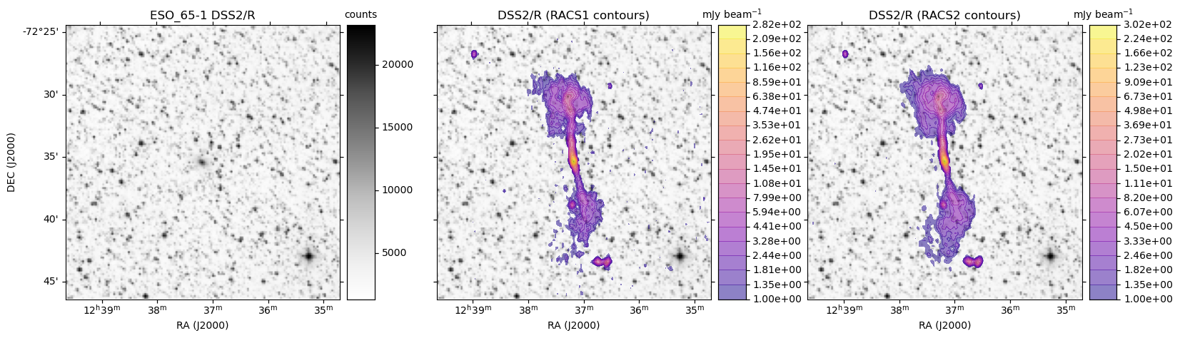
Radio overlays of ESO_65-1 ASKAP RACS images accessed directly from CASDA SIA and Datalink/SODA services.
Here we access the CASDA SIA and Datalink/SODA services to retrieve ASKAP RACS images directly from CASDA.
There are two examples on this page:
- The first downloads HiPS and RACS data before making some overlay plots.
- The second takes a simpler approach to just download the RACS data.
See this page for more details on how to access RACS data.
These images are more preferable for science applications compared to the RACS HiPS data used in our other HiPS and HiPS+MOC examples.
Note: You will need to input your own OPAL ATNF username and password for this script to work. Furthermore, there may be times the script does not work, e.g. when the services are undergoing maintenance.
from astropy.io.votable import parse_single_table
from io import BytesIO
import requests
from astropy.wcs import WCS
from mpl_toolkits.axes_grid1 import make_axes_locatable
import numpy as np
from astropy.io import fits
import matplotlib.pyplot as plt
import matplotlib as mpl
import re
from astropy.visualization import ImageNormalize, MinMaxInterval, AsinhStretch
from astropy import units as u
import os
from urllib.parse import quote
import multicolorfits as mcf

from requests.auth import HTTPBasicAuth
import warnings

warnings.filterwarnings('ignore', category=UserWarning, append=True)

#A function to make it easier to create a colorbar
#Adapted from https://joseph-long.com/writing/colorbars/
def colorbar(mappable,xlabel):
    last_axes = plt.gca()
    ax = mappable.axes
    fig = ax.figure
    divider = make_axes_locatable(ax)
    cax = divider.append_axes("right", size="10%", pad=0.1)
    #taking this approach to make a colorbar means the new axis is also of wcsaxes type
    #https://docs.astropy.org/en/stable/visualization/wcsaxes/
    #the following fixes up some issues and formats the colorbar
    cax.grid(False)
    cbar = fig.colorbar(mappable, cax=cax)
    cbar.ax.coords[1].set_ticklabel_position('r')
    cbar.ax.coords[1].set_auto_axislabel(False)
    cbar.ax.coords[0].set_ticks_visible(False)
    cbar.ax.coords[0].set_ticklabel_visible(False)
    cbar.ax.coords[1].set_axislabel(xlabel)
    cbar.ax.coords[1].set_axislabel_position('t')
    cbar.ax.coords[1].set_ticks_position('r')
    if(hasattr(mappable,'levels')):
        cbar.ax.coords[1].set_ticks(mappable.levels*u.dimensionless_unscaled)
        cbar.ax.coords[1].set_major_formatter('%.2e')
        #cbar.ax.coords[1].set_major_formatter('%.2f')
        cbar.ax.coords[1].set_ticklabel(exclude_overlapping=True)
    plt.sca(last_axes)
    return cbar

#A function to access the hips2fits service
#if the image is not empty, return the fits hdu
def get_hips_data(hips,pix_width, pix_height, diam, qra, qdec):
    url = 'http://alasky.u-strasbg.fr/hips-image-services/hips2fits?hips={}&width={}&height={}&fov={}&projection=TAN&coordsys=icrs&ra={}&dec={}&rotation_angle=0.0&format=fits'.format(quote(hips), pix_width, pix_height, diam*1.0/3600, qra, qdec)
    resp = requests.get(url)
    if(resp.status_code < 400):
        hdu = fits.open(BytesIO(resp.content))
        im = hdu[0].data
        if (not np.isnan(im[0][0])):
            return hdu
    else:
        return None

#A function to make each of the individual plots
#cnum = number of filled contour levels
#calpha = transparency of filled contours
def make_plot(ax,img,cimg,imlabel,clabel,pos,cnum = 20,calpha=0.5):
    #depending on where the image lies in the sequence (left, middle or right)
    #format the axes appropriately
    if(pos == 'l'):
        ax.coords[0].set_axislabel('RA (J2000)')
        ax.coords[1].set_axislabel('DEC (J2000)')

    if(pos == 'r'):
        ax.coords[1].set_ticklabel_position('r')
        ax.coords[1].set_axislabel_position('r')
        ax.coords[0].set_axislabel('RA (J2000)')
        ax.coords[1].set_axislabel('')
        ax.coords[1].set_auto_axislabel(False)
        ax.coords[1].set_ticklabel_visible(False)

    if(pos == 'm'):
         ax.coords[1].set_axislabel('')
         ax.coords[1].set_auto_axislabel(False)
         ax.coords[0].set_axislabel('RA (J2000)')
         ax.coords[1].set_ticklabel_visible(False)

    #plot the base image
    norm = ImageNormalize(img, interval=MinMaxInterval(),stretch=AsinhStretch())
    im = ax.imshow(img, cmap='Greys', norm=norm, origin='lower',aspect='auto')
    #add a colorbar from the base image if there is not a contour overlay to show
    if(cimg is None):
        #Add the colorbar and title
        colorbar(im,'counts')
        titre = imlabel
        ax.set_title(titre)
    else:
        #Get the min and max values from the contour image, ignoring nan values
        cmin = np.nanmin(cimg)
        cmax = np.nanmax(cimg)
        #If we have negative values, use a small number for the minimum
        if(cmin < 0):
            #1.0 mJy per beam
            cmin = 1e-3*1000
        #Determine the contours spaced equally in logspace
        cmin = np.log10(cmin)
        cmax = np.log10(cmax)
        clevels = np.logspace(cmin,cmax,cnum)
        #Choose a colour map
        cmap = mpl.cm.get_cmap('plasma')
        #Ensure that the full colour range is used via LogNorm
        norm = mpl.colors.LogNorm(vmin=10**cmin,vmax=10**cmax)
        #Create filled contours. Another option
        CS = ax.contourf(cimg,levels=clevels,cmap=cmap,alpha=calpha,norm=norm,origin='lower')
        #Add the colorbar and title
        colorbar(CS,'mJy beam$^{-1}$')
        titre = imlabel + " (%s contours)" % (clabel)
        ax.set_title(titre)

#URL for the CASDA SIA endpoint
url = "https://casda.csiro.au/casda_vo_tools/sia2/query"

#A few sample objects
#Query SIMBAD to get their coordinates
obj = 'ESO_65-1'
obj = 'Centaurus A'
obj = 'M83'
url = "http://simbad.u-strasbg.fr/simbad/sim-nameresolver?Ident=%s&output=json" % obj
simbad = requests.get(url).json()
qra = simbad[0]['ra']
qdec = simbad[0]['dec']

qrad=22/60*0.5
#ENTER YOUR OPAL USERNAME AND PASSWORD
#See https://opal.atnf.csiro.au/
opal_user='MY_OPAL_USERNAME'
opal_pass = 'MY_OPAL_PASSWORD'

if(opal_user == 'MY_OPAL_USERNAME' or opal_pass == 'MY_OPAL_PASSWORD'):
    print ('You did not set your ATNF OPAL username and password')
    exit()

#query the casda SIA service directly
#racs is under the COLLECTION 'The Rapid ASKAP Continuum Survey'
url = "https://casda.csiro.au/casda_vo_tools/sia2/query?POS=CIRCLE %s %s %s&COLLECTION=The Rapid ASKAP Continuum Survey&RESPONSEFORMAT=votable" % (qra,qdec,qrad)
vot = requests.get(url).content
table = parse_single_table(BytesIO(vot))
df = table.to_table(use_names_over_ids=True).to_pandas()
#only consider a subset of the available data useful for our purposes
df = df[(df['dataproduct_subtype'] == 'cont.restored.t0') & (df['pol_states']=='/I/')].reset_index()

#create a folder to save the fits files and the PNG plot
dload_dir = re.sub(" ","",obj) + "_racs"
if not os.path.exists(dload_dir):
    os.mkdir(dload_dir)

#a list to keep our useful images in
#we will also save the files to the above dload_dir
ilist = []

for idx in range(0,df.shape[0]):
    #access the datalink service for each of the SIA results
    #the datalink service returns a VOTable that contains the authenticated_id_token
    #needed to produce the image cutout from the casda SODA service
    #As we are interested in small images and for simplicity, we use the synchronous endpoint - sync -
    #of the SODA service (the asynchronous endpoint - async - could also be used)

    #only access the common resolution images
    #These are the second image type of RACS
    #see last paragraph of Section 3.4.2 of McConnell et al. 2020
    #https://ui.adsabs.harvard.edu/abs/2020PASA...37...48M/abstract
    #[To access the first image types, i.e. those not convolved to a common resolution,
    # change the following to 'cres in', to skip the cres images]
    if('cres' not in df.loc[idx,'filename']):
        continue

    #the url to the datalink service for the image of interest
    url = df.loc[idx,'access_url']
    #requires ATNF opal account to access
    links = requests.get(url,auth=HTTPBasicAuth(opal_user,opal_pass)).content
    links_df = parse_single_table(BytesIO(links)).to_table(use_names_over_ids=True).to_pandas()
    cutout = links_df[links_df['service_def'] == 'cutout_service'].reset_index()
    #get the token corresponding to the cutout service
    token = cutout.loc[0,'authenticated_id_token']
    #the url to download the fits data for the cutout
    soda_url = "https://casda.csiro.au/casda_data_access/data/sync?ID=%s&POS=CIRCLE %s %s %s" % (token,qra,qdec,qrad)
    print (soda_url)

    #try to download the image if it is not full of nan pixels
    fname = dload_dir + "/img%d.fits" % idx
    resp = requests.get(soda_url)
    if(resp.status_code < 400):
        hdu = fits.open(BytesIO(resp.content))
        im = hdu[0].data
        #check that we do not have any nan pixels in the image
        #since some of the SIA images may be empty, we have to check that here
        #Here we are interested only in images full of real pixels - so we use np.isnan(im).any()
        #If you wanted to include images with partial data (some real pixel data and some nan pixels),
        #then the following could be changed to 'if (not np.isnan(im).all()):'
        if(not np.isnan(im).any()):
            print (df.loc[idx,'filename']," GOOD ",idx)
            ilist.append(hdu)
            hdu.writeto(fname)
        else:
            print (df.loc[idx,'filename']," SKIPPING",idx)

#plot the resulting images...
if(len(ilist) > 0):
    #The figure size was chosen to ensure square images - adapt to number of results received (may be 1 or 2 or more per object)
    fsize=[19/3.0*(1+len(ilist)),5]
    #width of images in pixels (used by hips2fits service)
    pw = 150
    ph = pw
    diam = qrad * 3600 *2.0
    #first get the fits data
    base_hips = 'DSS2/R'
    print ("Getting ",base_hips)
    hdu_dss = get_hips_data(base_hips,pw,ph,diam,qra,qdec)
    #write out the dss image to file if needed
    #note - the width of the image is very small, so the spatial resolution will be low...
    #The hips2fits query could be altered to fix this: see http://alasky.u-strasbg.fr/hips-image-services/hips2fits
    hdu_dss.writeto(dload_dir + '/dssr.fits')
    #get the image data
    im_dss = hdu_dss[0].data
    #use the DSS image WCS for the projection for each panel
    custom = {}
    custom['projection'] = WCS(hdu_dss[0].header)
    #setup a plot with as many panels side by side as needed
    f, (axes) = plt.subplots(figsize=fsize,ncols=1+len(ilist),subplot_kw=custom)

    #make the first plot
    make_plot(axes[0],im_dss,None,obj + " " + base_hips,'',pos='l')
    nradio = 0
    for idx in range(0,len(ilist)):
        hdu_racs = ilist[idx]
        #reproject the data and rescale to mJy (multiply by 1000)
        #the '[0][0]' are needed to simplify the format of the RACS data for plotting
        img_racs  = mcf.reproject2D(hdu_racs[0].data[0][0],mcf.makesimpleheader(hdu_racs[0].header),hdu_dss[0].header)*1000
        #determine the position of the plot to add
        pos = 'm'
        if(nradio == len(ilist)-1):
            pos = 'r'
        title = 'RACS%d' % (idx+1)
        #make each radio image contour overlay plot
        make_plot(axes[idx+1],im_dss,img_racs,base_hips,title,pos=pos)
        hdu_racs.close()
        nradio = nradio + 1
    #save the file to disk
    ofile = dload_dir + '/plot.png'
    plt.savefig(ofile,bbox_inches='tight')
    plt.close()
    hdu_dss.close()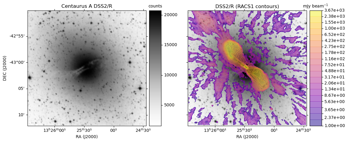
Radio overlays of Centaurus A ASKAP RACS images accessed directly from CASDA SIA and Datalink/SODA services.
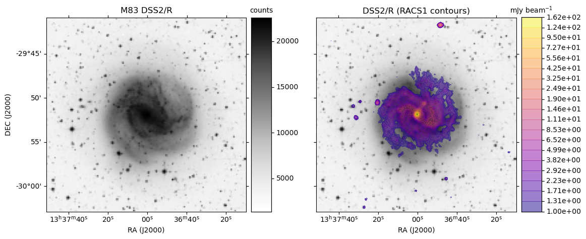
Radio overlays of M83 ASKAP RACS images accessed directly from CASDA SIA and Datalink/SODA services.
This second example focuses only on downloading the data, either for a single object or a list of objects in a csv file:
#contents of sample_list.csv used in the following example
#name,ra,dec
NGC6337,17:22:15.67,-38:29:01.73
NGC5189,13:33:32.88,-65:58:27.04
from astropy.io.votable import parse_single_table
from io import BytesIO
import requests
from requests.auth import HTTPBasicAuth
import numpy as np
from astropy.io import fits
import re
import os
from astropy import units as u
from astropy.io import ascii
import astropy.coordinates as coord
#object name, ra, dec and radius (0.5*fov) of image in degrees
def get_racs(qobj,qra,qdec,qrad):
#URL for the CASDA SIA endpoint
url = "https://casda.csiro.au/casda_vo_tools/sia2/query"
#ENTER YOUR OPAL USERNAME AND PASSWORD
#See https://opal.atnf.csiro.au/
opal_user='MY_OPAL_USERNAME'
opal_pass = 'MY_OPAL_PASSWORD'
if(opal_user == 'MY_OPAL_USERNAME' or opal_pass == 'MY_OPAL_PASSWORD'):
print ('You did not set your ATNF OPAL username and password')
exit()
#query the casda SIA service directly
#racs is under the COLLECTION 'The Rapid ASKAP Continuum Survey'
url = "https://casda.csiro.au/casda_vo_tools/sia2/query?POS=CIRCLE %s %s %s&COLLECTION=The Rapid ASKAP Continuum Survey&RESPONSEFORMAT=votable" % (qra,qdec,qrad)
vot = requests.get(url).content
table = parse_single_table(BytesIO(vot))
df = table.to_table(use_names_over_ids=True).to_pandas()
#only consider a subset of the available data useful for our purposes
df = df[(df['dataproduct_subtype'] == 'cont.restored.t0') & (df['pol_states']=='/I/')].reset_index()
#create a folder to save the fits files and the PNG plot
dload_dir = re.sub(" ","",qobj) + "_racs"
if not os.path.exists(dload_dir):
os.mkdir(dload_dir)
for idx in range(0,df.shape[0]):
#access the datalink service for each of the SIA results
#the datalink service returns a VOTable that contains the authenticated_id_token
#needed to produce the image cutout from the casda SODA service
#As we are interested in small images and for simplicity, we use the synchronous endpoint - sync -
#of the SODA service (the asynchronous endpoint - async - could also be used)
#only access the common resolution images
#These are the second image type of RACS
#see last paragraph of Section 3.4.2 of McConnell et al. 2020
#https://ui.adsabs.harvard.edu/abs/2020PASA...37...48M/abstract
#[To access the first image types, i.e. those not convolved to a common resolution,
# change the following to 'cres in', to skip the cres images]
if('cres' not in df.loc[idx,'filename']):
continue
#the url to the datalink service for the image of interest
url = df.loc[idx,'access_url']
#requires ATNF opal account to access
links = requests.get(url,auth=HTTPBasicAuth(opal_user,opal_pass)).content
links_df = parse_single_table(BytesIO(links)).to_table(use_names_over_ids=True).to_pandas()
cutout = links_df[links_df['service_def'] == 'cutout_service'].reset_index()
#get the token corresponding to the cutout service
token = cutout.loc[0,'authenticated_id_token']
#the url to download the fits data for the cutout
soda_url = "https://casda.csiro.au/casda_data_access/data/sync?ID=%s&POS=CIRCLE %s %s %s" % (token,qra,qdec,qrad)
print (soda_url)
#try to download the image if it is not full of nan pixels
fname = dload_dir + "/img%d.fits" % idx
resp = requests.get(soda_url)
if(resp.status_code < 400):
hdu = fits.open(BytesIO(resp.content))
im = hdu[0].data
#check that we do not have any nan pixels in the image
#since some of the SIA images may be empty, we have to check that here
#Here we are interested only in images full of real pixels - so we use np.isnan(im).any()
#If you wanted to include images with partial data (some real pixel data and some nan pixels),
#then the following could be changed to 'if (not np.isnan(im).all()):'
if(not np.isnan(im).any()):
print (df.loc[idx,'filename']," GOOD ",idx)
hdu.writeto(fname)
else:
print (df.loc[idx,'filename']," SKIPPING",idx)
#Retrieve RACS data for single object
#We use simbad to resolve its name to get the coordinates
#A few sample objects
#Query SIMBAD to get their coordinates
qobj = 'ESO_65-1'
qobj = 'Centaurus A'
qobj = 'M83'
url = "http://simbad.u-strasbg.fr/simbad/sim-nameresolver?Ident=%s&output=json" % qobj
simbad = requests.get(url).json()
qra = simbad[0]['ra']
qdec = simbad[0]['dec']
#22 arcmin fov
qrad=22/60*0.5
get_racs(qobj,qra,qdec,qrad)
#Alternatively, read in coordinates of objects from a CSV
tbl = ascii.read('sample_list.csv')
#get racs for each object in sample_list.csv
for row in tbl:
obj_name = row[0]
ra = coord.Angle(row[1],unit=u.hour)
dec = coord.Angle(row[2],unit=u.degree)
#4 arcmin FOV
rad = 4/60*0.5
print ("Retrieving RACS data for ",obj_name)
get_racs(obj_name,ra.degree,dec.degree,rad)