
Colour mosaic with radio contour overlay
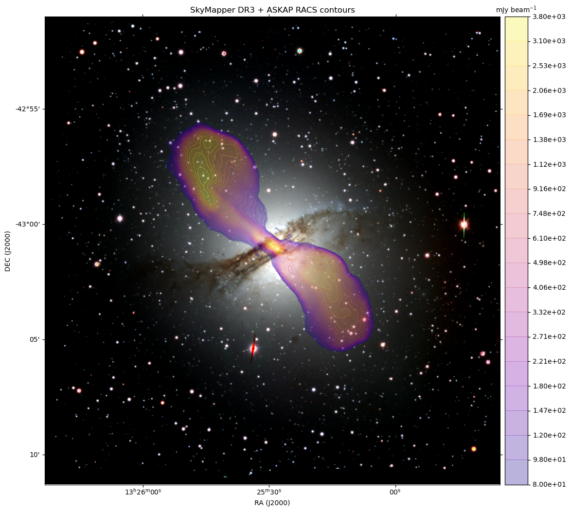
SkyMapper DR3 mosaic of Centaurus A as a colour-composite image with red = i-band, green = r-band and blue = g-band. Contours are from ASKAP RACS. Field of view is 0.3 deg.
In this example we plot a colour-composite image made from large SkyMapper mosaics of Cen A using the MontagePy code of another example. Added as an overlay are radio contours from the HiPS format ASKAP RACS data that were downloaded using the hips2fits service (see also this example).
Note: Since the images used here are from SkyMapper DR3, we do not provide them for download.
Please see this example for code to produce your own large mosaics.
This example forms part of a series of General Virtual Observatory Examples developed by Data Central.
import matplotlib.pyplot as plt
import matplotlib as mpl
import numpy as np
from astropy.io import fits
from astropy.wcs import WCS
from mpl_toolkits.axes_grid1 import make_axes_locatable
import requests
import multicolorfits as mcf
from astropy import units as u
import os

#A function to make it easier to create a colorbar
#Adapted from https://joseph-long.com/writing/colorbars/
def colorbar(mappable,xlabel):
    last_axes = plt.gca()
    ax = mappable.axes
    fig = ax.figure
    divider = make_axes_locatable(ax)
    cax = divider.append_axes("right", size="5%", pad=0.1)
    #taking this approach to make a colorbar means the new axis is also of wcsaxes type
    #https://docs.astropy.org/en/stable/visualization/wcsaxes/
    #the following fixes up some issues and formats the colorbar
    cax.grid(False)
    cbar = fig.colorbar(mappable, cax=cax)
    cbar.ax.coords[1].set_ticklabel_position('r')
    cbar.ax.coords[1].set_auto_axislabel(False)
    cbar.ax.coords[0].set_ticks_visible(False)
    cbar.ax.coords[0].set_ticklabel_visible(False)
    cbar.ax.coords[1].set_axislabel(xlabel)
    cbar.ax.coords[1].set_axislabel_position('t')
    cbar.ax.coords[1].set_ticks_position('r')
    if(hasattr(mappable,'levels')):
        cbar.ax.coords[1].set_ticks(mappable.levels*u.dimensionless_unscaled)
        cbar.ax.coords[1].set_major_formatter('%.2e')
        #cbar.ax.coords[1].set_major_formatter('%.2f')
        cbar.ax.coords[1].set_ticklabel(exclude_overlapping=True)
    plt.sca(last_axes)
    return cbar

#Pre-made SkyMapper mosaics
#see https://docs.datacentral.org.au/help-center/virtual-observatory-examples/skymapper-siamontage-multiple-position-query-mosaics/
#for Python code : mosaic size = 0.3 deg
rimg=fits.open('CenA/i.fits')[0]
gimg=fits.open('CenA/r.fits')[0]
bimg=fits.open('CenA/g.fits')[0]

#RACS image pre-downloaded using
#http://alasky.u-strasbg.fr/hips-image-services/hips2fits
#with https://www.atnf.csiro.au/research/RACS/RACS_I1/ in the 'HiPS survey' input field.
racs = fits.open('CenA/racs.fits')[0]

#ensure all images are matching the green image (r-band) by reprojecting them
rimg = mcf.reproject2D(rimg.data,mcf.makesimpleheader(rimg.header),gimg.header)
bimg = mcf.reproject2D(bimg.data,mcf.makesimpleheader(bimg.header),gimg.header)
#contours
cimg = mcf.reproject2D(racs.data,mcf.makesimpleheader(racs.header),gimg.header)*1000

rdata = rimg.data
gdata = gimg.data
bdata = bimg.data

gamma = 1.0
locut=45
hicut=99.5
#create the colour image using mcf
gr = mcf.greyRGBize_image(rdata,min_max=[locut,hicut],rescalefn='asinh',scaletype='perc',gamma=gamma,checkscale=False)
gg = mcf.greyRGBize_image(gdata,min_max=[locut,hicut],rescalefn='asinh',scaletype='perc',gamma=gamma,checkscale=False)
gb = mcf.greyRGBize_image(bdata,min_max=[locut,hicut],rescalefn='asinh',scaletype='perc',gamma=gamma,checkscale=False)
cr = mcf.colorize_image(gr,(255,0,0),colorintype='rgb',gammacorr_color=gamma)
cg = mcf.colorize_image(gg,(0,255,0),colorintype='rgb',gammacorr_color=gamma)
cb = mcf.colorize_image(gb,(0,0,255),colorintype='rgb',gammacorr_color=gamma)
img = mcf.combine_multicolor([cr,cg,cb],gamma=gamma)
wcs = WCS(gimg.header)

#choose a large image size
fsize=[19*1/3*2.5,5*2.5]
custom = {}
custom['projection'] = wcs
#We use subplots here as our other examples used it
f, (ax1) = plt.subplots(figsize=fsize,ncols=1,subplot_kw=custom)
ax1.imshow(img,origin='lower')

#cmin = np.nanmin(cimg)
cmax = np.nanmax(cimg)
#set min to 80 mJy to focus on the lobes
cmin = 80
cnum=20
#Determine the contours spaced equally in logspace
cmin = np.log10(cmin)
cmax = np.log10(cmax)
clevels = np.logspace(cmin,cmax,cnum)
#Choose a colour map
cmap = mpl.cm.get_cmap('plasma')
#Transparency of the contours
calpha=0.3
#Ensure that the full colour range is used via LogNorm
norm = mpl.colors.LogNorm(vmin=10**cmin,vmax=10**cmax)
#Create filled contours.
CS = ax1.contourf(cimg,levels=clevels,cmap=cmap,alpha=calpha,norm=norm,origin='lower')
#Add the colorbar and title
colorbar(CS,'mJy beam$^{-1}$')
#titre = imlabel + " (%s contours)" % (clabel)
ax1.set_title('SkyMapper DR3 + ASKAP RACS contours')
ax1.coords[0].set_axislabel('RA (J2000)')
ax1.coords[1].set_axislabel('DEC (J2000)')
#write the image to a PNG
plt.savefig('CenA.png',bbox_inches='tight')
plt.show()