
SSA: Fitting Gaussian Emission Lines in Time Series Spectra
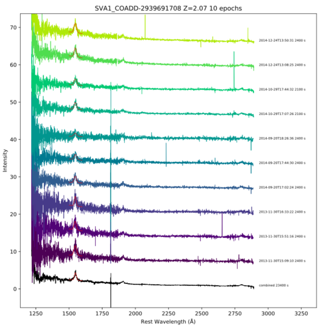
Gaussian fits to the emission line CIV 1550 in SVA1_COADD-2939691708

The FWHM of the above Gaussian fits to CIV 1550. Blue points represent individual measurements and the line indicates the measurement for the combined spectrum.
Here we expand on the Plotting Time Series Ozdes Spectra example and fit a Gaussian to the CIV 1550 A emission line in SVA1_COADD-2939691708.
We use the LMFIT Python module to construct and fit a Gaussian + Line model to the data.
The below figures show the generated output plots.
See the LMFIT examples page for more info.
from specutils import Spectrum1D
import matplotlib.pyplot as plt
import matplotlib as mpl
from matplotlib.backends.backend_pdf import PdfPages
import pandas as pd
from astropy.stats import sigma_clip
from astropy.table import QTable

import requests
from io import BytesIO

from astropy.time import Time
from astropy import units as u
import numpy as np
import os
from pyvo.dal.ssa  import search, SSAService
#LMFIT: see https://lmfit.github.io/lmfit-py/builtin_models.html#gaussianmodel
from lmfit.models import GaussianModel,VoigtModel,LorentzianModel,SkewedGaussianModel,LinearModel

url = "https://datacentral.org.au/vo/ssa/query"
service = SSAService(url)

#A region with ozdes spectra. RA=55 deg; Dec=-29.1 deg
qra=55
qdec=-29.1
pos = (qra*u.deg,qdec*u.deg)
fsize=[10,10]

mpl.rcParams['axes.linewidth'] = 0.7
LWIDTH=0.5

custom = {}
#diameter of search around qra,qdec = 0.5 degrees
#increase SIZE to 1.0 to get a lot more nearby targets to plot
custom['SIZE'] = 0.5
#restrict our focus to only ozdes spectra
custom['COLLECTION'] = 'ozdes_dr2'
custom['TARGETNAME'] ='SVA1_COADD-2939691708'

#if needed, you can specify one target of interest
#custom['TARGETNAME'] = 'DES13C2acs'
#custom['TARGETNAME'] = 'SVA1_COADD-2939694059'
#custom['TARGETNAME'] = 'SVA1_COADD-2939675022'

#perform the SSA query using pyvo
results = service.search(pos=pos,**custom)

#convert results to a pandas dataframe
df =results.votable.get_first_table().to_table(use_names_over_ids=True).to_pandas()

#how many rows...
nrows = df.shape[0]
print (nrows, " rows of results received")

#Select the output format
#PDF = single PDF with separate pages per target (can be a little cpu intensive to draw)
OUTPUT_FORMAT = "PDF"

#We will plot each target in a separate page of the output ozdes.pdf
#Stacking the spectra vertically in a similar fashion to specplot in IRAF
if("PDF" in OUTPUT_FORMAT):
    pdf = PdfPages('fit_results.pdf')

#Get a list of the unique targets received in the results
uniq_targ = df['target_name'].unique()

#Choose a colour map to display our spectra
#see https://matplotlib.org/3.1.0/tutorials/colors/colormaps.html for other colourmaps
#cmap = mpl.cm.get_cmap('plasma')
cmap = mpl.cm.get_cmap('viridis')

#some variables to store the results of the Gaussian fits
mjd = []
fwhm = []
fwhm_err = []

combined_fwhm = None
combined_fwhm_err = None

for targ in uniq_targ:
    #Here we create a subset dataframe for each target, listing all the spectra belonging to targ
    #We sort by dataproduct_subtype and mid-exposure time to ensure the combined spectrum is first, followed
    #by all other spectra in order of increasing mid-exposure time of each observation
    #We call reset_index to ensure that the subset dataframe is freshly indexed from 0 to ... NSPEC
    #to make it easier to iterate over the subset dataframe
    subset = df[(df['target_name'] == targ)].sort_values(by=['dataproduct_subtype','t_midpoint']).reset_index()
    NSPEC = subset.shape[0]
    #Only include targets with several spectra to plot
    if(NSPEC > 10):
        print (NSPEC,targ)
        #vertical offset between each spectrum; set below...
        offset = None
        #used to choose the colour of the spectrum, depending on its vertical position
        norm = mpl.colors.Normalize(vmin=1,vmax=NSPEC)
        redshift = None
        #reset the plot for each new target
        plt.figure(figsize=fsize)
        yval_combined = None
        wave_combined = None
        flux_combined = None
        #go through each spectrum of the target
        for idx in range(0,NSPEC):
            #We have to add the RESPONSEFORMAT here to get fits results...
            url = subset.loc[idx,'access_url']+"&RESPONSEFORMAT=fits"
            print ("Downloading spectrum ",idx, " of ",NSPEC-1)
            #retrieve the spectrum. Note we are not writing it to disk in this example
            spec = Spectrum1D.read(BytesIO(requests.get(url).content),format='wcs1d-fits')
            nspec = len(spec.spectral_axis)
            waves = spec.wavelength
            wave_label ="Wavelength ($\mathrm{\AA}$)"

            #if the combined spectrum has a defined redshift, store it
            #and use it for all other spectra
            #We also correct the wavelength scale to the rest wavelength frame
            if(idx == 0 and subset.loc[idx,'redshift'] >= 0):
                redshift = subset.loc[idx,'redshift']
            if(redshift is not None):
                waves = waves/(1+redshift)
                wave_label ="Rest Wavelength ($\mathrm{\AA}$)"

            #for the combined spectrum, get its clipped range, so we can determine the y limits to
            #guide plotting for all the spectra.
            #Note that are we only using the sigma_clip function to get the y limits and we plot the
            #original spectra

            #plot the combined spectrum in black; otherwise, use the colour as indicated above
            if(idx == 0):
                clipped = sigma_clip(spec[int(0+0.01*nspec):int(nspec-0.01*nspec)].flux,masked=False,sigma=10)
                ymin = min(clipped).value
                ymax = max(clipped).value
                offset = (ymax-ymin)*0.5
                #median of flux in last 90-95% of spectrum for label placement
                yval_combined = np.median(spec[int(0+0.90*nspec):int(nspec-0.05*nspec)].flux.value)
                plt.plot(waves,spec.flux+idx*offset*u.Unit('ct/Angstrom'),'k-',linewidth=LWIDTH)
                #save combined spectrum so we can replot it at the end.
                wave_combined = waves
                flux_combined = spec.flux+idx*offset*u.Unit('ct/Angstrom')
                #setup some other overall plot things
                #don't need to multiply by u.Unit('ct/Angstrom') since it is just matplotlib numbers
                plt.ylim(ymin,ymax+(NSPEC-1)*offset)
                x1,x2 = plt.xlim()
                #set the xrange a little wider on the right side, to allow for the labelling of each spectrum
                plt.xlim(x1,x2*1.13)
                #Set a title. Adding the redshift if available
                titre = "%s %d epochs" % (targ,subset.loc[idx,'t_xel'])
                if(redshift is not None):
                    titre = "%s Z=%.2f %d epochs" % (targ,subset.loc[idx,'redshift'],subset.loc[idx,'t_xel'])
                plt.title(titre)
            else:
                plt.plot(waves,spec.flux+idx*offset*u.Unit('ct/Angstrom'),color=cmap(norm(idx)),linewidth=LWIDTH)

            #labelling of each spectrum with the mid-exposure time of observation and exposure time
            tmid = Time(subset.loc[idx,'t_midpoint'],format='mjd')
            tmid.format='isot'
            label = tmid.value[:-4]
            if(idx == 0):
                label = "combined"
            label = label + " " + str(int(subset.loc[idx,'t_exptime'])) + " s"
            #plot the label at the right of the spectrum
            plt.text(waves[nspec-1].value*1.01,yval_combined+idx*offset,label,ha='left',verticalalignment='center',fontsize=6)
            plt.xlabel(wave_label)
            plt.ylabel("Intensity")

            #plot the combined spectrum again, to ensure it is not overplotted by other spectra
            #if(wave_combined is not None):
            #    plt.plot(wave_combined,flux_combined,'k-',linewidth=LWIDTH)

            #FIT the CIV 1550 emission line with a Gaussian

            #focus on region around line of interest
            #Note we use an astropy QTable here, as converting both wavelength and flux to
            #pandas directly from Spectrum1D is problematic (big vs small endian issues)
            sdf = QTable({ "wave": waves, "flux": spec.flux}).to_pandas()
            #restrict the range to the line of interest
            sdf = sdf[(sdf['wave'] >= 1500.0) & (sdf['wave'] <= 1600.0)]
            #remove any null values which upset LMFIT
            sdf = sdf[sdf.flux.notna()]

            #a Gaussian function is good for the purposes of this demo
            v1 = GaussianModel(prefix="v1_")

            x=np.array(sdf['wave'])
            y=np.array(sdf['flux'])

            pars = v1.guess(y,x=x)

            #Add a line to the model for the continuum
            line1 = LinearModel(prefix="l1_")
            pars.update(line1.make_params())
            #get the continuum level
            cont = np.average(sdf[(sdf['wave'] >= 1580) & (sdf['wave'] <= 1590)]['flux'])

            pars['l1_slope'].set(0)
            #important to set the continuum level here to guide the fit
            pars['l1_intercept'].set(cont)


            #our model is a sum of the Gaussian and the straight line
            mod = v1 + line1
            #fit the model to the data
            out = mod.fit(y,pars,x=x)

            #keep some FWHM values to plot...but keep one from combined spectrum separate
            if(idx > 0):
                mjd.append(subset.loc[idx,'t_midpoint'])
                fwhm.append(out.params['v1_fwhm'].value)
                fwhm_err.append(out.params['v1_fwhm'].stderr)

            if(idx == 0):
                combined_fwhm = out.params['v1_fwhm'].value
                combined_fwhm_err = out.params['v1_fwhm'].stderr

            plt.plot(sdf['wave'],out.best_fit+idx*offset,'r-',linewidth=LWIDTH)#*0.75)

        #optionally show the plot interactively
        #plt.show()
        #save the plot to the pdf file
        if("PDF" in OUTPUT_FORMAT):
            pdf.savefig()

        plt.close()

plt.figure()

#Create a plot of the FWHM measurements
plt.errorbar(mjd,fwhm,yerr=fwhm_err,fmt='o')
plt.title("CIV 1550")
plt.xlabel("Modified Julian Day (d)")
plt.ylabel("Full-Width at Half-Maximum ($\mathrm{\AA}$)")
x1,x2 = plt.xlim()
#plot the measurement from the combined spectrum as a line
plt.plot([x1-x1*0.1,x2+x2*0.1],[combined_fwhm,combined_fwhm],'k-',linewidth=LWIDTH)
plt.plot([x1-x1*0.1,x2+x2*0.1],[combined_fwhm+combined_fwhm_err,combined_fwhm+combined_fwhm_err],'k--',linewidth=LWIDTH)
plt.plot([x1-x1*0.1,x2+x2*0.1],[combined_fwhm-combined_fwhm_err,combined_fwhm-combined_fwhm_err],'k--',linewidth=LWIDTH)
#adjust the limits to stick to the spectral range
plt.xlim(x1,x2)
pdf.savefig()
plt.close()


#close the pdf file
if("PDF" in OUTPUT_FORMAT):
    pdf.close()