SSA: GALAH DR3 Interactive Spectra Explorer enhanced by the Data Central API
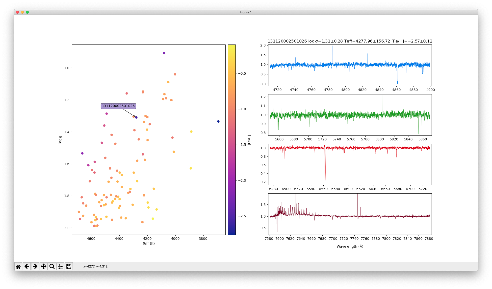
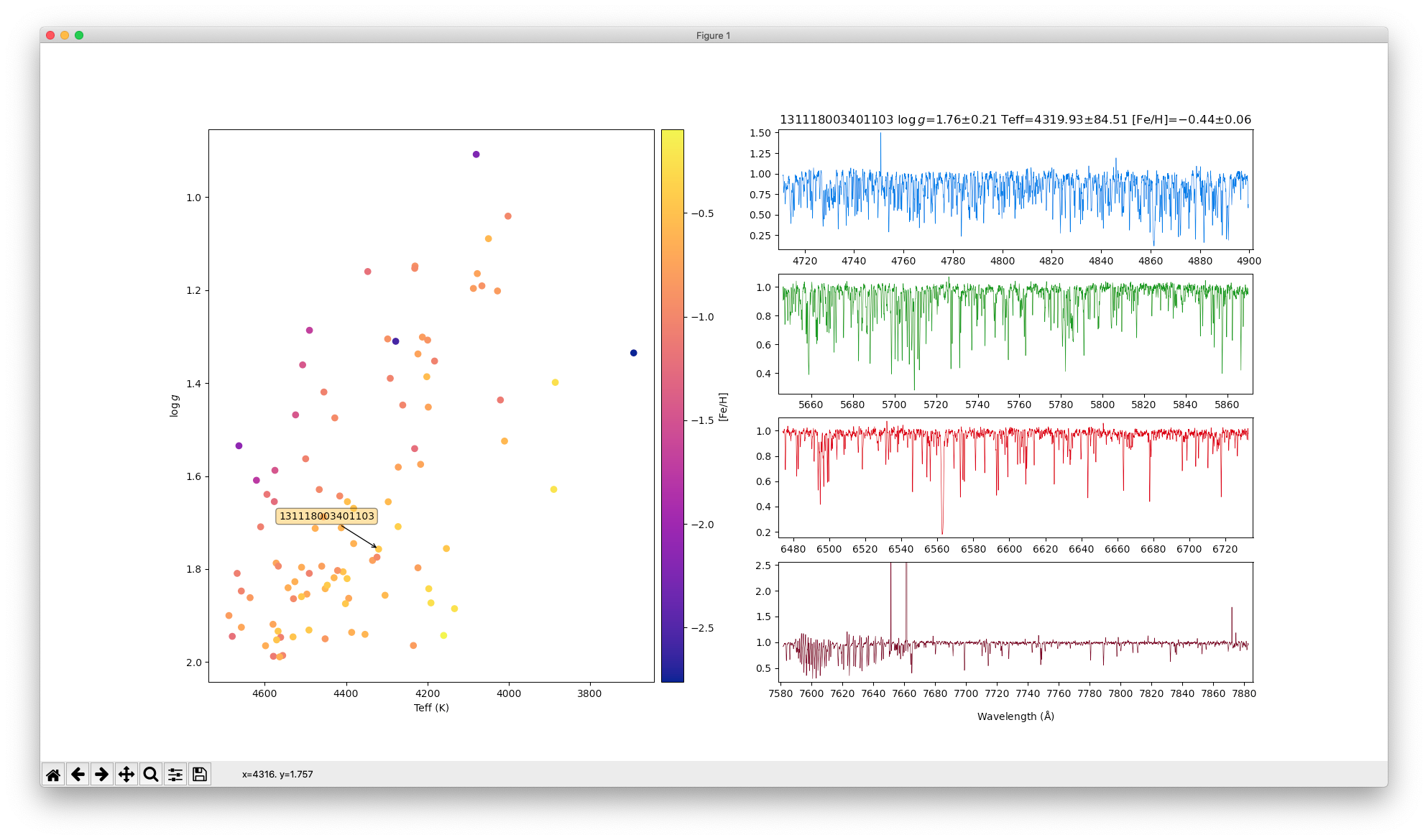
In this example we take a slightly approach to accessing the GALAH DR3 spectra. Instead of using the SSA service to acquire GALAH DR3 target details, we use the DataCentral API to query the GALAH DR3 tables directly using an ADQL query. The SSA service is then used to retrieve the relevant spectra on demand.
Please note that this interactive version was developed to be run from running the Python script directly on MacOSX (tested on 10.14 and 10.15).
It is not intended to be executed from within a Python notebook.
Instructions: Run the script (you may need to resize the window for the plot to scale correctly) and then click on points to plot their spectra.
from specutils import Spectrum1D
import matplotlib.pyplot as plt
import matplotlib as mpl
from matplotlib.backends.backend_pdf import PdfPages
from matplotlib import gridspec
from mpl_toolkits.axes_grid1 import make_axes_locatable
import numpy as np
import pandas as pd
import matplotlib.ticker as plticker
from astropy.stats import sigma_clip
from astropy.time import Time
import requests
import re
from io import BytesIO
from astropy import units as u
from pyvo.dal.ssa  import search, SSAService

#called by onpick to retrieve and show the spectra of the target of interest
def show_spectrum(name,axes,title):
    #query the SSA service
    #no position required as we already know the target name from the DataCentral API query
    url = "https://datacentral.org.au/vo/ssa/query"
    service = SSAService(url)
    custom = {}
    custom['TARGETNAME'] = name
    custom['COLLECTION'] = 'galah_dr3'
    results = service.search(**custom)
    df = results.votable.get_first_table().to_table(use_names_over_ids=True).to_pandas()
    filters = ['B','V','R','I']
    colours = ["#085dea","#1e8c09","#cf0000","#640418"]

    #go through each filter and plot its spectrum (if available)
    for idx in range(0,4):
        filt = filters[idx]
        ax = axes[idx]
        #remove any previous spectrum/labels/titles that may have been plotted in a previous call of
        #the show_spectrum function
        ax.clear()
        #show the title in the first position only
        if(idx == 0):
            ax.set_title(title)
        #select only the spectrum of the filter of interest
        subset = df[(df['band_name'] == filt)].reset_index()
        #give preference to using the continuum normalised spectra
        if(subset[subset['dataproduct_subtype'].isin(['normalised'])].shape[0] > 0):
            subset = subset[(subset['dataproduct_subtype'] == "normalised")].reset_index()
        #only proceed if we have the filter of interest available in the results
        if(subset.shape[0] > 0):
            #add RESPONSEFORMAT=fits here to ensure we get fits format back
            url= subset.loc[0,'access_url'] + "&RESPONSEFORMAT=fits"
            #load the spectrum
            spec = Spectrum1D.read(BytesIO(requests.get(url).content),format='wcs1d-fits')
            exptime = subset.loc[0,'t_exptime']
            ax.tick_params(axis='both', which='major')
            ax.tick_params(axis='both', which='minor')
            loc = plticker.MultipleLocator(base=20.0)
            ax.xaxis.set_major_locator(loc)
            #plot label at last position (caveat: no check if spectra are missing)
            if(idx == 3):
                ax.set_xlabel("Wavelength ($\mathrm{\AA}$)",labelpad=10)
            #plot the spectrum
            ax.plot(spec.wavelength,spec.flux,linewidth=LWIDTH,color=colours[idx])
            #adjust the y-scale to best fit the spectrum with some sigma clipping
            nspec = len(spec.spectral_axis)
            clipped = sigma_clip(spec[int(0+0.01*nspec):int(nspec-0.01*nspec)].flux,masked=False,sigma=15)
            ymin = min(clipped).value
            ymax = max(clipped).value
            xmin = spec.wavelength[0].value
            xmax = spec.wavelength[nspec-1].value
            #add a 1% buffer either side of the x-range
            dx=0.01*(xmax-xmin)
            ax.set_xlim(xmin-dx,xmax+dx)
            #add a 1% buffer either side of the y-range
            dy=0.03*(ymax-ymin)
            ax.set_ylim(ymin-dy,ymax+dy)
        #else:
            #print missing data...

#set the figure size to be wide in the horizontal direction
#to accommodate the image cutouts alongside the spectra
fsize=[20,13]
mpl.rcParams['axes.linewidth'] = 0.7
FSIZE=18
LWIDTH=0.5
LABELSIZE=10

#Instead of querying SSA directly, we query the galah_dr3 table main_star
#using the DataCentral API
#Information about the table can be found at
#https://docs.datacentral.org.au/galah/dr3/catalogue-data-access/
# and
#https://docs.datacentral.org.au/galah/dr3/table-schema/
# and
#https://datacentral.org.au/services/schema/#galah.dr3.catalogues.mainstargroup.main_star

#Here we select the top 100 sources with names < 160000000000000 and low surface gravities (log g < 2)
#together with their temperatures, surface gravities and metallicities
sql_query = "SELECT TOP 100 sobject_id, star_id, teff,e_teff,logg,e_logg, fe_h, e_fe_h FROM galah_dr3.main_star WHERE sobject_id < 160000000000000 and logg < 2.0"
#Query GALAH DR3 catalogue using DataCentral API
api_url = 'https://datacentral.org.au/api/services/query/'
qdata = {'title' : 'galah_test_query',
         'notes' : 'test query for ssa example',
         'sql' : sql_query,
         'run_async' : False,
         'email'  : 'brent.miszalski@mq.edu.au'}
post = requests.post(api_url,data=qdata).json()
resp = requests.get(post['url']).json()
#convert the results to a pandas dataframe
df = pd.DataFrame(resp['result']['data'],columns=resp['result']['columns'])
#remove results where the teff and logg are not determined
#as the dataframe entries are still all strings, we have to do the following
#instead of use nona() or notnull() functions of the dataframe
df = df[(df['teff'] != "nan") & (df['logg'] != "nan")]
#convert columns to floats - needed since data coming from json results
convertme = ['teff','e_teff','logg','e_logg','fe_h','e_fe_h']
for c in convertme:
    df[c] = df[c].astype(float)
print (df)
#create a few lists/arrays to conveniently access the results
teff = np.array(df['teff'])
teff_err = np.array(df['e_teff'])
logg = np.array(df['logg'])
logg_err = np.array(df['e_logg'])
fe_h = np.array(df['fe_h'])
fe_h_err = np.array(df['e_fe_h'])
names = np.array(df['sobject_id'])

#create a colourmap tied to the metallicity ([Fe/H])
cmap = mpl.cm.get_cmap('plasma')
norm = mpl.colors.Normalize(vmin=min(fe_h),vmax=max(fe_h))

#setup the plot using gridspec
gs = gridspec.GridSpec
fig = plt.figure(figsize=fsize)
#4 rows, 2 cols
#plot of log g/Teff takes up first col (all rows)
#spectra take up all rows of 2nd col
gs = gridspec.GridSpec(4,2)
ax1 = fig.add_subplot(gs[:,0])
#B
axB = fig.add_subplot(gs[0,1])
#V
axV = fig.add_subplot(gs[1,1])
#R
axR = fig.add_subplot(gs[2,1])
#I
axI = fig.add_subplot(gs[3,1])

#plot the location of the results in a log g vs teff diagram
#with the colours of each point determined by the [Fe/H] and the colourmap
#The picker argument is required to allow for picking targets interactively (see below)
sc = ax1.scatter(teff,logg,cmap=cmap,c=fe_h,picker=5)

#create some space for the colourbar and add it
divider = make_axes_locatable(ax1)
cax = divider.append_axes('right',size='5%',pad=0.1)
fig.colorbar(mappable=sc,label='[Fe/H]',cax=cax)

#this annotation is a template for a label that appears when the mouse hovers
#over each point in the above scatter plot
annot = ax1.annotate("",xy=(0,0),xytext=(-100,30),textcoords="offset points",
        bbox=dict(boxstyle="round",fc="w"),
        arrowprops=dict(arrowstyle="->"))
#all are off by default
annot.set_visible(False)

#flip y axis to show lower surface gravity at top
ax1.invert_yaxis()
#flip x axis to show cooler stars at right
ax1.invert_xaxis()
#set the axis labels
ax1.set_ylabel("$\\log\\,g$")
ax1.set_xlabel("Teff (K)")

#function to update the annotations
def update_annot(ind):
    pos = sc.get_offsets()[ind["ind"][0]]
    annot.xy = pos
    text = "%s" % [names[n] for n in ind["ind"]][0]
    annot.set_text(text)
    annot.get_bbox_patch().set_facecolor(cmap(norm(fe_h[ind["ind"][0]])))
    annot.get_bbox_patch().set_alpha(0.5)

#called when the mouse hovers over a target
def hover(event):
    vis = annot.get_visible()
    if event.inaxes == ax1:
        cont, ind = sc.contains(event)
        if cont:
            update_annot(ind)
            annot.set_visible(True)
            fig.canvas.draw_idle()
        else:
            if vis:
                annot.set_visible(False)
                fig.canvas.draw_idle()

#called when the user clicks a target
def onpick(event):
    ind = event.ind
    pt = event.artist.get_offsets()
    #mouse positions
    mx = event.mouseevent.xdata
    my = event.mouseevent.ydata
    #get closest index to mouse click
    #chosen contains the index of the
    #closest target to the mouse click
    dist = 1e6
    chosen = None
    for idx in ind:
        print (idx)
        print (pt[idx])
        px = pt[idx][0]
        py = pt[idx][1]
        d = np.sqrt((px-mx)**2 + (py-my)**2)
        if(d < dist):
            print ("names[%d]" % idx,d)
            chosen = idx
            dist = d

    if(chosen is not None):
        print (names[chosen],chosen)
        #set a title that shows some of the information extracted from the API query
        #this information is not part of the SSA obscore metadata
        titre = "%s $\\log\\,g$=%.2f$\\pm$%.2f Teff=%.2f$\\pm$%.2f [Fe/H]=%.2f$\\pm$%.2f" % (names[chosen],
                logg[chosen],logg_err[chosen],
                teff[chosen],teff_err[chosen],
                fe_h[chosen],fe_h_err[chosen])
        #make the - sign in [Fe/H] proper if needed
        titre = re.sub("-","$-$",titre)
        #make the spectrum show up in the right panels
        show_spectrum(names[chosen],[axB,axV,axR,axI],titre)


#make sure the events are setup
fig.canvas.mpl_connect("motion_notify_event",hover)
fig.canvas.mpl_connect("pick_event",onpick)
plt.show()

