
SSA: Plotting Time Series OzDES Spectra
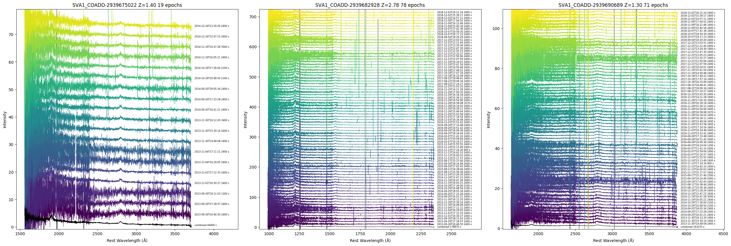
Output of the above script for three different ozdes_dr2 targets
In this example we plot time series spectra from OzDES DR2 in a similar fashion to the specplot task in IRAF.
from specutils import Spectrum1D
import matplotlib.pyplot as plt
import matplotlib as mpl
from matplotlib.backends.backend_pdf import PdfPages
import pandas as pd
from astropy.stats import sigma_clip

import requests
from io import BytesIO

from astropy.time import Time
from astropy import units as u
import numpy as np
import os
from pyvo.dal.ssa  import search, SSAService

url = "https://datacentral.org.au/vo/ssa/query"
service = SSAService(url)

#A region with ozdes spectra. RA=55 deg; Dec=-29.1 deg
qra=55
qdec=-29.1
pos = (qra*u.deg,qdec*u.deg)
fsize=[10,10]

mpl.rcParams['axes.linewidth'] = 0.7
LWIDTH=0.5

custom = {}
#diameter of search around qra,qdec = 0.5 degrees
#increase SIZE to 1.0 to get a lot more nearby targets to plot
custom['SIZE'] = 0.2
#restrict our focus to only ozdes spectra
custom['COLLECTION'] = 'ozdes_dr2'
#if needed, you can specify one target of interest
#custom['TARGETNAME'] = 'DES13C2acs'
#custom['TARGETNAME'] = 'SVA1_COADD-2939694059'
#custom['TARGETNAME'] = 'SVA1_COADD-2939675022'

#perform the SSA query using pyvo
results = service.search(pos=pos,**custom)

#convert results to a pandas dataframe
df =results.votable.get_first_table().to_table(use_names_over_ids=True).to_pandas()

#how many rows...
nrows = df.shape[0]
print (nrows, " rows of results received")

#Select the output format
#PNG = single PNG per target (fast preview)
#PDF = single PDF with separate pages per target (can be a little cpu intensive to draw)
OUTPUT_FORMAT = "PNG"
#OUTPUT_FORMAT = "PDF"

#We will plot each target in a separate page of the output ozdes.pdf
#Stacking the spectra vertically in a similar fashion to specplot in IRAF
if("PDF" in OUTPUT_FORMAT):
    pdf = PdfPages('ozdes.pdf')

#Get a list of the unique targets received in the results
uniq_targ = df['target_name'].unique()

#Choose a colour map to display our spectra
#see https://matplotlib.org/3.1.0/tutorials/colors/colormaps.html for other colourmaps
#cmap = mpl.cm.get_cmap('plasma')
cmap = mpl.cm.get_cmap('viridis')

for targ in uniq_targ:
    #Here we create a subset dataframe for each target, listing all the spectra belonging to targ
    #We sort by dataproduct_subtype and start time to ensure the combined spectrum is first, followed
    #by all other spectra in order of increasing start time of each observation
    #We call reset_index to ensure that the subset dataframe is freshly indexed from 0 to ... NSPEC
    #to make it easier to iterate over the subset dataframe
    subset = df[(df['target_name'] == targ)].sort_values(by=['dataproduct_subtype','t_min']).reset_index()
    NSPEC = subset.shape[0]
    #Only include targets with several spectra to plot
    if(NSPEC > 10):
        print (NSPEC,targ)
        #vertical offset between each spectrum; set below...
        offset = None
        #used to choose the colour of the spectrum, depending on its vertical position
        norm = mpl.colors.Normalize(vmin=1,vmax=NSPEC)
        redshift = None
        #reset the plot for each new target
        plt.figure(figsize=fsize)
        yval_combined = None
        wave_combined = None
        flux_combined = None
        #go through each spectrum of the target
        for idx in range(0,NSPEC):
            #We have to add the RESPONSEFORMAT here to get fits results...
            url = subset.loc[idx,'access_url']+"&RESPONSEFORMAT=fits"
            print ("Downloading spectrum ",idx, " of ",NSPEC-1)
            #retrieve the spectrum. Note we are not writing it to disk in this example
            spec = Spectrum1D.read(BytesIO(requests.get(url).content),format='wcs1d-fits')
            nspec = len(spec.spectral_axis)
            waves = spec.wavelength
            wave_label ="Wavelength ($\mathrm{\AA}$)"

            #if the combined spectrum has a defined redshift, store it
            #and use it for all other spectra
            #We also correct the wavelength scale to the rest wavelength frame
            if(idx == 0 and subset.loc[idx,'redshift'] >= 0):
                redshift = subset.loc[idx,'redshift']
            if(redshift is not None):
                waves = waves/(1+redshift)
                wave_label ="Rest Wavelength ($\mathrm{\AA}$)"

            #for the combined spectrum, get its clipped range, so we can determine the y limits to
            #guide plotting for all the spectra.
            #Note that are we only using the sigma_clip function to get the y limits and we plot the
            #original spectra

            #plot the combined spectrum in black; otherwise, use the colour as indicated above
            if(idx == 0):
                clipped = sigma_clip(spec[int(0+0.01*nspec):int(nspec-0.01*nspec)].flux,masked=False,sigma=10)
                ymin = min(clipped).value
                ymax = max(clipped).value
                offset = (ymax-ymin)*0.5
                #median of flux in last 90-95% of spectrum for label placement
                yval_combined = np.median(spec[int(0+0.90*nspec):int(nspec-0.05*nspec)].flux.value)
                plt.plot(waves,spec.flux+idx*offset*u.Unit('ct/Angstrom'),'k-',linewidth=LWIDTH)
                #save combined spectrum so we can replot it at the end.
                wave_combined = waves
                flux_combined = spec.flux+idx*offset*u.Unit('ct/Angstrom')
                #setup some other overall plot things
                #don't need to multiply by u.Unit('ct/Angstrom') since it is just matplotlib numbers
                plt.ylim(ymin,ymax+(NSPEC-1)*offset)
                x1,x2 = plt.xlim()
                #set the xrange a little wider on the right side, to allow for the labelling of each spectrum
                plt.xlim(x1,x2*1.13)
                #Set a title. Adding the redshift if available
                titre = "%s %d epochs" % (targ,subset.loc[idx,'t_xel'])
                if(redshift is not None):
                    titre = "%s Z=%.2f %d epochs" % (targ,subset.loc[idx,'redshift'],subset.loc[idx,'t_xel'])
                plt.title(titre)
            else:
                plt.plot(waves,spec.flux+idx*offset*u.Unit('ct/Angstrom'),color=cmap(norm(idx)),linewidth=LWIDTH)

            #labelling of each spectrum with the start time of observation and exposure time
            tstart = Time(subset.loc[idx,'t_min'],format='mjd')
            tstart.format='isot'
            label = tstart.value[:-4]
            if(idx == 0):
                label = "combined"
            label = label + " " + str(int(subset.loc[idx,'t_exptime'])) + " s"
            #plot the label at the right of the spectrum
            plt.text(waves[nspec-1].value*1.01,yval_combined+idx*offset,label,ha='left',verticalalignment='center',fontsize=6)
            plt.xlabel(wave_label)
            plt.ylabel("Intensity")

        #plot the combined spectrum again, to ensure it is not overplotted by other spectra
        if(wave_combined is not None):
            plt.plot(wave_combined,flux_combined,'k-',linewidth=LWIDTH)

        #optionally show the plot interactively
        #plt.show()
        #save the plot to the pdf file
        if("PDF" in OUTPUT_FORMAT):
            pdf.savefig()
        if("PNG" in OUTPUT_FORMAT):
            ofname = targ + ".png"
            print ("Writing out ",ofname)
            plt.savefig(ofname,bbox_inches='tight')

        plt.close()

#close the pdf file
if("PDF" in OUTPUT_FORMAT):
    pdf.close()