
SSA: GALAH DR3
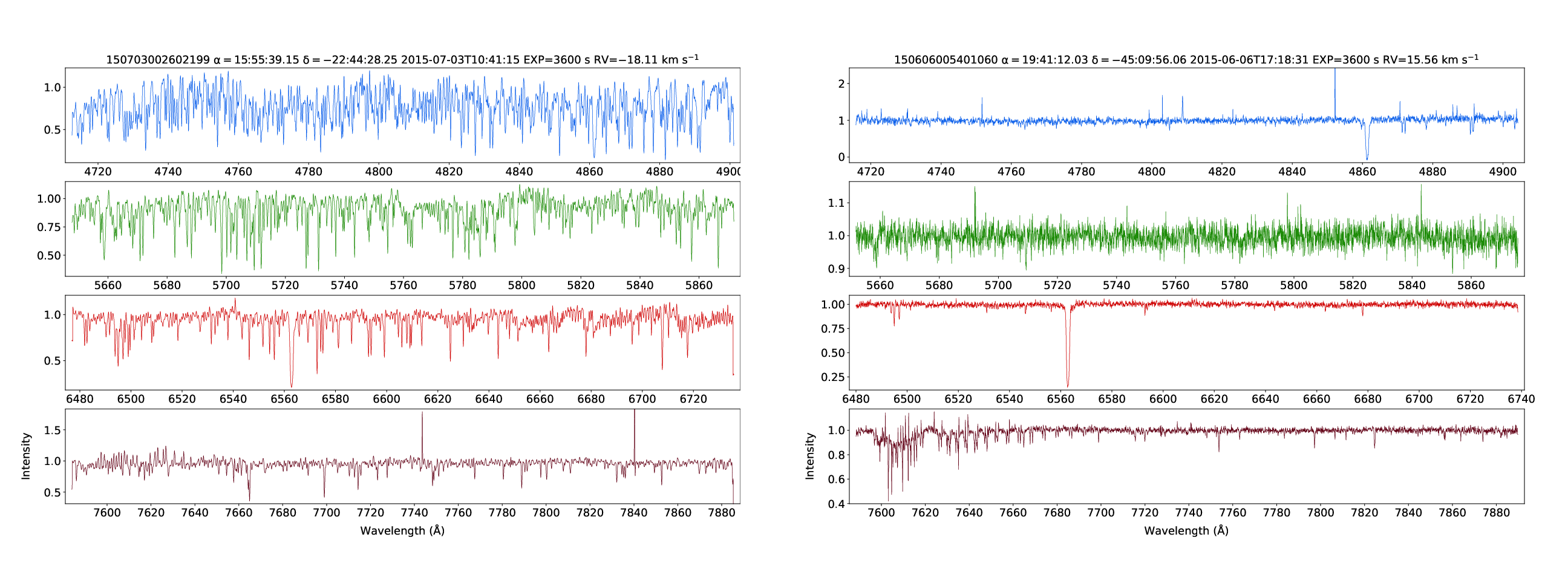
GALAH DR3 spectra of a relatively metal-rich star (150703002602199, [Fe/H]=1.00) and a relatively metal-poor star (150606005401060, [Fe/H]=-2.90).
This example queries the SSA service directly to plot GALAH DR3 spectra from each arm of the Hermes spectrograph in a single plot.
from specutils import Spectrum1D
import astropy.coordinates as coord
import matplotlib.pyplot as plt
import matplotlib as mpl
from matplotlib.backends.backend_pdf import PdfPages
from matplotlib import gridspec
import pandas as pd
import matplotlib.ticker as plticker
from astropy.stats import sigma_clip
from astropy.time import Time
import requests
import re
from io import BytesIO
from astropy import units as u
from pyvo.dal.ssa  import search, SSAService

##set the figure size to be wide in the horizontal direction
fsize=[20,13]
mpl.rcParams['axes.linewidth'] = 0.7
FSIZE=18
LWIDTH=0.5

#URL of the SSA service
url = "https://datacentral.org.au/vo/ssa/query"
service = SSAService(url)
indiv_results = []
targets = ['150606005401060','150703002602199']
#since SSA does not support more than one value per each parameter
#to query multiple targets we perform separate queries
#and append the results to indiv_results in the form of pandas dataframes
#Once done, we can concatenate the results into a single dataframe
#that makes processing the results a lot easier
#Note that we exclude the pos parameter here, since we are using the targetname
for t in targets:
    custom = {}
    custom['TARGETNAME'] = t
    #only retrieve the normalised spectra
    custom['DPSUBTYPE'] = 'normalised'
    custom['COLLECTION'] = 'galah_dr3'
    results = service.search(**custom)
    indiv_results.append(results.votable.get_first_table().to_table(use_names_over_ids=True).to_pandas())

#dataframe containing all our results
df = pd.concat(indiv_results,ignore_index=True)

i = 0

plotidx = 0
PLOT=1
ofname = 'galah.pdf'
print ("Writing results to: ",ofname)
pdf = PdfPages(ofname)

uniq_targ = df['target_name'].unique()
#spectra that we want to plot, corresponding to each arm of the HERMES spectrograph
filters = ['B','V','R','I']

for targ in uniq_targ:
    #setup a new plot for each object
    f = plt.figure(figsize=fsize)
    print (targ)

    running = 0
    #get the number of spectra to retrieve for the target of interest
    tdf = df[(df['target_name'] == targ)]
    NSPEC = tdf[tdf['band_name'].isin(filters)].shape[0]
    for filt in filters:
        subset = df[(df['target_name'] == targ) & (df['band_name'] == filt)].sort_values(by=['band_name']).reset_index()
        #We use gridspec to lay out the expected number of elements
        gs = gridspec.GridSpec(NSPEC,1)
        gs.update(wspace=0.1)
        #In some cases one of the different arm's spectra are missing (e.g. the I-band)
        if(subset.shape[0] > 0):
            #need to add RESPONSEFORMAT=fits here to get fits format returned
            url= subset.loc[0,'access_url'] + "&RESPONSEFORMAT=fits"
            print ("Downloading ",url)
            #read the spectrum in using specutils
            spec = Spectrum1D.read(BytesIO(requests.get(url).content),format='wcs1d-fits')
            #read the exposure time from the dataframe that contains all the obscore parameters
            exptime = subset.loc[0,'t_exptime']

            #setup the subplot containing the spectrum
            ax = plt.subplot(gs[running,0])
            ax.tick_params(axis='both', which='major', labelsize=FSIZE)
            ax.tick_params(axis='both', which='minor', labelsize=FSIZE)

            #set 20-Angstrom tickmarks
            loc = plticker.MultipleLocator(base=20.0)
            ax.xaxis.set_major_locator(loc)
            if(running == NSPEC-1):
                ax.set_xlabel("Wavelength ($\mathrm{\AA}$)",labelpad=10,fontsize=FSIZE)
                ax.set_ylabel("Intensity",labelpad=20,fontsize=FSIZE)
            #select the colour of the line depending on which spectrum we are plotting
            colour = None

            if(subset.loc[0,'band_name'] == "B"):
                colour = "#085dea"
            if(subset.loc[0,'band_name'] == "V"):
                colour = "#1e8c09"
            if(subset.loc[0,'band_name'] == "R"):
                colour = "#cf0000"
            if(subset.loc[0,'band_name'] == "I"):
                colour = "#640418"

            #plot the spectrum
            ax.plot(spec.wavelength,spec.flux,linewidth=LWIDTH,color=colour)

            #now work out the best y-axis range to plot
            #use sigma clipping to determine the limits, but exclude 1 per cent of the wavelength range
            #at each end of the spectrum (often affected by noise or other systematic effects)
            nspec = len(spec.spectral_axis)
            clipped = sigma_clip(spec[int(0+0.01*nspec):int(nspec-0.01*nspec)].flux,masked=False,sigma=15)
            ymin = min(clipped).value
            ymax = max(clipped).value
            xmin = spec.wavelength[0].value
            xmax = spec.wavelength[nspec-1].value
            #add a 1% buffer either side of the x-range
            dx=0.01*(xmax-xmin)
            ax.set_xlim(xmin-dx,xmax+dx)
            #add a 1% buffer either side of the y-range
            dy=0.03*(ymax-ymin)
            ax.set_ylim(ymin-dy,ymax+dy)
            #get some basic information for a title
            #from the SSA obscore information
            #more information can be obtaining querying the galah_dr3
            #table directly using the DataCentral API (see other SSA example)
            target = "%s" % subset.loc[0,'target_name']
            tmid = Time(subset.loc[0,'t_midpoint'],format='mjd')
            tmid.format='isot'
            #Add the title if the first plotted spectrum
            if(running == 0):
                rc = coord.Angle(subset.loc[0,'s_ra'],unit=u.degree)
                dc = coord.Angle(subset.loc[0,'s_dec'],unit=u.degree)
                coords = "$\mathrm{\\alpha=}$%s $\mathrm{\\delta=}$%s" % (rc.to_string(unit=u.hour,sep=':')[:-2],dc.to_string(unit=u.deg,sep=':')[:-2])
                coords = re.sub("-","$-$",coords)
                titre = "%s %s %s EXP=%s s" % (target,coords,tmid.value[:-4],int(exptime))
                #not all spectra have the RV defined in the SSA obscore output
                if(subset.loc[0,'rv'] != ""):
                    rvstr = " RV=%.2f" % subset.loc[0,'rv']
                    titre = titre + re.sub("-","$-$",rvstr) + " km s$^{-1}$"
                ax.set_title(titre,fontsize=FSIZE)

            running = running + 1
    pdf.savefig()
    #plt.show()
    plt.close()

pdf.close()