SIA Examples - Data Central

Simple Image Access Examples

Simple Image Access (SIA) service

This page details more advanced usage of the SIA service. The examples provided below utilise one or more of the following:

Python (astropy and pyvo modules)
ds9 and pyds9
Aladin
TOPCAT

Please refer to the accompanying page:

Data Central SIA service

for details on the parameters and basic usage.

Please contact us if any of the following is unclear or you require further assistance in using the SIA2 service.

Access from Python

The SIA service can be accessed from your own Python scripts in various ways.

This page contains some example approaches with Python 3 that may be useful.

Relatively quick access: Retrieving and parsing a VOTABLE

An outline of the steps may be as follows:

Create a string containing your query request.
Send the request and download the VOTABLE results to a file.
Open (parse) the VOTABLE file and extract the download links to each image cutout.
Create wget commands to download the cutouts.

An example Python script is provided below. It requires the astropy module to be installed.

from astropy.io.votable import parse_single_table
import requests

#SIA2 query URL
#Devils
url = "https://datacentral.org.au/vo/sia2/query?FORMAT=fits&POS=CIRCLE 150 2.2 0.05"
#GAMA
#url = "https://datacentral.org.au/vo/sia2/query?FORMAT=fits&POS=CIRCLE 217.4 0.25 0.05"

#filename to store the results of the query
vot = 'test_table.xml'
#perform the query
r = requests.get(url)
#write the results of the query
fptr = open(vot,'wb')
fptr.write(r.content)
fptr.close()
#open the table with astropy's votable package
table = parse_single_table(vot)
data = table.array

#Go through each row in the table
for i in range (0,len(data)):
    obs_id = str(data['obs_id'][i],'utf-8')
    obs_collection = str(data['obs_collection'][i],'utf-8')
    facility_name =  str(data['facility_name'][i],'utf-8')
    band_name = str(data['band_name'][i],'utf-8')
    #URL of the cutout
    access_url = str(data['access_url'][i],'utf-8')
    #filename to download to
    ofname = "%s-%s-%s-%s.fits" % (obs_id,obs_collection, facility_name,band_name)
    #print out a wget command to download the data
    download_cmd = "wget -O %s \"%s\"" % (ofname,access_url)
    print (download_cmd)

More advanced access: Using the pyvo module

An outline of the steps may be as follows:

Read in a file containing coordinates of several objects of interest.
Use the pyvo SIA2 service interface to construct a query
Send a query for each object with the ability to easily specify multiple parameters
Download the query results into a separate folder for each object

An example object list (sample_list.csv) and Python script are provided below.

Important: To enable SIA2 access you must have installed the latest development version of the pyvo module from the pyvo github page.

You may need to uninstall any previous pyvo installations you have before installing the latest version.

#name,ra,dec
galaxy1,10:00:11.838,+2:13:50.050
galaxy2,9:59:51.066,+2:12:36.742
galaxy3,10:00:00.125,+2:11:06.359
galaxy4,10:00:08.935,+2:09:57.920

import astropy.coordinates as coord
from astropy import units as u
from astropy.io import ascii
import os
#You must have the latest version of the pyvo module that has sia2 support
from pyvo.dal.sia2 import search, SIAService, SIAQuery

#URL for the AAO DataCentral SIA2 service
url = "https://datacentral.org.au/vo/sia2/query"
service = SIAService(url)

#Read in coordinates of four objects from a CSV
tbl = ascii.read('sample_list.csv')

#we request 1 arcmin square images
image_radius = 30.0/3600

#for each object
for row in tbl:
    obj_name = row[0]
    ra = coord.Angle(row[1],unit=u.hour)
    dec = coord.Angle(row[2],unit=u.degree)
    #position and radius to query 
    pos = (ra.degree*u.deg,dec.degree*u.deg,image_radius*u.deg)

    #Now setup some additional parameters. 
    #Other examples: see test_sia2_remote.py in the pyvo source code
    
    #Option 1: specify the desired images using the band parameter
    #results = service.search(pos=pos,band=(500e-9,800e-9))

    #Option 2: use the custom parameter FILTER to specify the filter names
    #Since it is a custom parameter, we have to pass it to **kwargs parameter of search() with the 'custom' dictionary
    filters = ['g','r','i']
    custom= {}
    custom['FILTER'] = filters
    #Mid-infrared example:
    #filters = ['IRAC1','IRAC2','IRAC3','IRAC4']
    #custom['FACILITY'] = 'Spitzer'
    #Perform the query
    results = service.search(pos=pos,**custom)

    #Make a folder based on each object name
    if not os.path.exists(obj_name):
        os.mkdir(obj_name)

    #Retrieve FITS image cutouts for the object
    for image in results:
        #filename is the Filter name (band_name); Since 'band_name' is not an ObsCore standard field, we access it differently
        fname = "%s/%s.fits" % (obj_name,str(image['band_name'],'utf-8'))
        #An optional filename combining Facility (facility_name) and Filter name
        #fname = "%s/%s%s.fits" % (obj_name,image.facility_name,str(image['band_name'],'utf-8'))
        #An optional longer filename if desired
        #fname = "%s/%s-%s-%s-%s.fits" % (obj_name,image.obs_id,image.obs_collection,image.facility_name,str(image['band_name'],'utf-8'))
        #Download the data
        print ("Downloading %s..." % fname)
        image.cachedataset(filename=fname)

    #Retrieve PNG preview images of each frame too
    #the query remains the same, but we add FORMAT='png' and some other PNG related parameters
    #Even though FORMAT is a standard parameter, we have to add it to custom to get it to work correctly
    custom['FORMAT'] = 'png'
    custom['PNG_CMAP'] = 'afmhot'
    custom['PNG_TITLE'] = 'True'

    #Perform the query 
    results = service.search(pos=pos,**custom)
    
    #Retrieve PNG image cutouts for the object
    for image in results:
        #filename is the Filter name (band_name)
        fname = "%s/%s.png" % (obj_name,str(image['band_name'],'utf-8'))
        #An optional filename combining Facility (facility_name) and Filter name
        #fname = "%s/%s%s.png" % (obj_name,image.facility_name,str(image['band_name'],'utf-8'))
        #An optional longer filename if desired
        #fname = "%s/%s-%s-%s-%s.png" % (obj_name,image.obs_id,image.obs_collection,image.facility_name,str(image['band_name'],'utf-8'))
        #Download the data
        print ("Downloading %s..." % fname)
        image.cachedataset(filename=fname)

#The downloaded files are arranged as follows
$ ls -r galaxy* 
galaxy4:
r.png	r.fits	i.png	i.fits	g.png	g.fits

galaxy3:
r.png	r.fits	i.png	i.fits	g.png	g.fits

galaxy2:
r.png	r.fits	i.png	i.fits	g.png	g.fits

galaxy1:
r.png	r.fits	i.png	i.fits	g.png	g.fits

Incorporating the pyds9 module

We can extend the above example to visualise the FITS images using ds9 and the pyds9 module.

If not installed already, you will need to install the ds9 FITS viewer (webpage) and the pyds9 module (github page).

The following Python code could be run after the above script.

The pyds9 module allows you to interact with ds9 using the powerful, low-level XPA access point commands.

import re
import pyds9
#load ds9
d = pyds9.DS9()
#remove any frames already in ds9
d.set("frame delete all")
#our list of object names
obj = ["galaxy1","galaxy2","galaxy3","galaxy4"]
#for each object
for o in obj:
    #create a new RGB frame and load up each colour separately
    d.set("frame new rgb")
    d.set("rgb red")
    d.set("file %s/i.fits" % o)
    d.set("rgb green")
    d.set("file %s/r.fits" % o)
    d.set("rgb blue")
    d.set("file %s/g.fits" % o)
    #lock the scale to allow the scale to be altered
    d.set("rgb lock scale yes")
    #get the image dimensions
    dim = re.split(" ",d.get("fits size"))
    tx = 0.30*int(dim[0])
    ty = 0.77*int(dim[1])
    #add an object name label in top left corner 
    reg = "image; text %s %s # text=%s font=\"times 16\"" % (tx,ty,o)
    d.set("regions",reg)
#set the frame display to tiled to show all images
d.set("tile yes")
d.set("frame 1")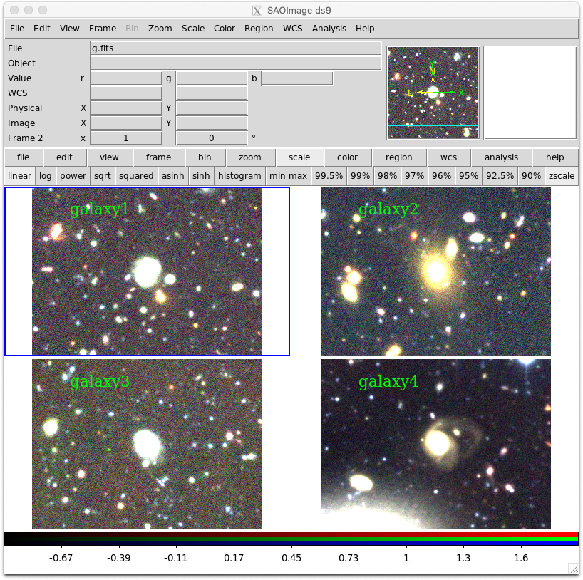

Example usage of pyds9 to visualise SIA service image cutouts from a Python script.

Using pyds9 to visualise multiple wavebands for a single object

We can adopt a similar approach to visualising multiple filter images for a single object.

The following Python script also aligns each image using the world coordinate system matching capability of ds9.

import astropy.coordinates as coord
from astropy import units as u
from astropy.io import ascii
import os
import re
import pyds9
d = pyds9.DS9()
#You must have the latest version of the pyvo module that has sia2 support
from pyvo.dal.sia2 import search, SIAService, SIAQuery

#URL for the AAO DataCentral SIA2 service
url = "https://datacentral.org.au/vo/sia2/query"
service = SIAService(url)

#Read in coordinates of four objects from a CSV
tbl = ascii.read('sample_list.csv')

#we request 1 arcmin square images
image_radius = 30.0/3600

#for each object
for row in tbl:
    obj_name = row[0]
    if(obj_name == "galaxy2"):
        ra = coord.Angle(row[1],unit=u.hour)
        dec = coord.Angle(row[2],unit=u.degree)
        #position and radius to query 
        pos = (ra.degree*u.deg,dec.degree*u.deg,image_radius*u.deg)

        #specify facilities. leaving out UKIRT.
        #easiest to use this custom dict
        custom= {}
        facilities = ['CFHT','VISTA','GALEX','Spitzer']
        custom['FACILITY'] = facilities

        results = service.search(pos=pos,band=(100e-9,8000e-9),**custom)

        #Make a folder based on each object name
        if not os.path.exists(obj_name):
            os.mkdir(obj_name)

        #start ds9 here
        #the downloaded images will appear as they are downloaded
        d = pyds9.DS9()
        d.set("frame delete all")
        d.set("tile yes")

        #Retrieve FITS image cutouts for the object
        for image in results:
            facility_name = image.facility_name
            band_name = str(image['band_name'],'utf-8')
            label = "%s %s" % (facility_name,band_name)
            #filename is the Filter name (band_name)
            fname = "%s/%s.fits" % (obj_name,band_name)
            #Download the data
            print ("Downloading %s..." % fname)
            image.cachedataset(filename=fname)
            #load the image if not CFHT NIR
            if(label != "CFHT H" and label != "CFHT K"):
                d.set("frame new")
                d.set("file %s" % fname)
                #set bb as the colourmap
                d.set("cmap bb")
                #set scale to be linear and 99.5%
                d.set("scale linear")
                d.set("scale mode 99.5")
                #add a 10" radius circle region around the object
                #also include a text label with the facility and filter with the circle
                print ("label: ",label)
                reg = "fk5; circle %sd %sd 10\"# text={%s} font=\"times 16\"" % (ra.degree,dec.degree,label)
                d.set("regions",reg)
            
        #tidy up the layout; match wcs using image in frame 4
        d.set("frame 4")
        d.set("match frame wcs")
        d.set("tile yes")
        d.set("frame 1")
        d.set("view magnifier no")
        d.set("view panner no")
        d.set("view info no")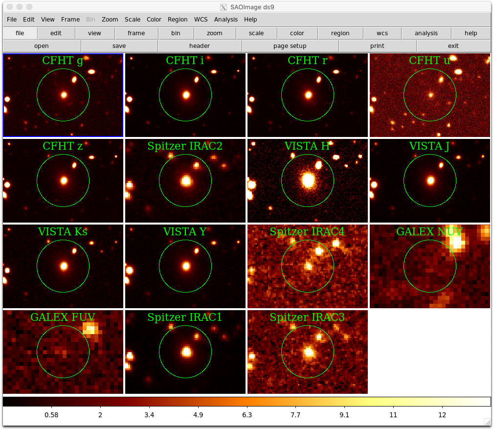

Example usage of pyds9 to visualise SIA service image cutouts for a single object from a Python script.

Interacting with the Single Object Viewer (SOV)

We can extend the above examples by incorporating results from the Simple Cone Search (SCS) service to identify objects of interest located within a retrieved SIA image cutout. In the following we download some images, perform a SCS query and overlay the results using ds9 regions. Some additional code allows us to interactively select objects to load in the Single Object Viewer (SOV) web page again using the XPA access point commands and pyds9.

To explore objects in the image, put your cursor near the object and press one of the following keys:

's' to load SAMI DR2 data in the SOV (near red circles),
'g' to load GAMA DR2 in the SOV (near yellow circles),
'w' to query SIMBAD (anywhere)
'q' to quit.

import pyds9 
from astropy.io.votable import parse_single_table
from astropy.coordinates import SkyCoord
import astropy.coordinates as coord

import astropy.units as u
import pyvo 
from pyvo.dal.sia2 import SIAService
import re
import os

#URL for the AAO DataCentral SIA2 service
sia_url = "https://datacentral.org.au/vo/sia2/query"
sia_service = SIAService(sia_url)

#Retrieve the 6 arcmin square images
image_radius = 180.0/3600

obj_name = 'interactive'
qra=217.45103	
qdec=0.28289
ra_cen = coord.Angle(qra,unit=u.degree)
dec_cen = coord.Angle(qdec,unit=u.degree)
#position and radius to query 
sia_pos = (ra_cen.degree*u.deg,dec_cen.degree*u.deg,image_radius*u.deg)

#Option 2: use the custom parameter FILTER to specify the filter names
#Since it is a custom parameter, we have to pass it to **kwargs parameter of search() with the 'custom' dictionary
filters = ['g','r','i']
custom= {}
custom['FILTER'] = filters
custom['FACILITY'] = 'VST'
#Perform the query
results = sia_service.search(pos=sia_pos,**custom)

#Make a folder based on each object name
if not os.path.exists(obj_name):
    os.mkdir(obj_name)

#Retrieve FITS image cutouts for the object
for image in results:
    #filename is the Filter name (band_name); Since 'band_name' is not an ObsCore standard field, we access it differently
    fname = "%s/%s.fits" % (obj_name,str(image['band_name'],'utf-8'))
    print ("Downloading %s..." % fname)
    if not os.path.exists(fname):
        image.cachedataset(filename=fname)

#Now that we have the data, let's load a colour image

d=pyds9.DS9()
d.set("frame delete all")
d.set("frame new rgb")
d.set("rgb red")
d.set("file %s/i.fits" % obj_name)
d.set("rgb green")
d.set("file %s/r.fits" % obj_name)
d.set("rgb blue")
d.set("file %s/g.fits" % obj_name)
d.set("rgb lock scale yes")
d.set("scale mode 99")

#Perform the SCS query
scs_table = pyvo.dal.conesearch(
        "https://datacentral.org.au/vo/cone-search/",
        SkyCoord(ra=ra_cen,dec=dec_cen),
        radius=image_radius*1.3*3600*u.arcsec)
#Print the results to the terminal
print (scs_table)
#Display the results as regions in the image
for row in scs_table:
    ra = row['RA ICRS']
    dec = row['DEC ICRS']
    dcid = row['DC ID']
    if(row['Dataset'] == 'SAMI DR2'):
        reg = "fk5;circle %sd %sd 5\"# text={%s} font=\"times 10\" color=red" % (ra,dec,dcid)
        d.set("regions",reg)
    elif(row['Dataset'] == 'GAMA DR2'):
        reg = "fk5;circle %sd %sd 10\"# text={%s} font=\"times 10\" color=yellow" % (ra,dec,dcid)
        d.set("regions",reg)

#Zoom out to see the whole image
d.set("zoom to fit")

#Interactive loop to allow for loading each object in the Data Central SOV 
while True:
    print ("Press:\n\t's' near a red circle (SAMI DR2)\n\t'g' near a yellow circle (GAMA DR2)\n\t'w' to query SIMBAD\n\t'q' to quit interactive mode.")
    inp = d.get("iexam key coordinate fk5 degrees") 
    dat = re.split(" ",inp)
    dataset = None
    if(dat[0] == 'q'):
        break
    if(dat[0] == 'g'):
        dataset = 'GAMA DR2'
    if(dat[0] == 's'):
        dataset = 'SAMI DR2'
    if(dataset != None):
        #cursor position
        cursor = SkyCoord(ra=dat[1]+"d",dec=dat[2]+"d")
        #Only consider objects less than 15 arcsec from cursor
        min_dist = 15.0
        min_id = None
        for row in scs_table:
            obj_ra = "%.6fd" % row['RA ICRS']
            obj_dec = "%.6fd" % row['DEC ICRS']
            obj = SkyCoord(ra=obj_ra,dec=obj_dec)
            sep = cursor.separation(obj)
            if(sep.arcsec < min_dist and row['Dataset'] == dataset):
                min_dist = sep.arcsec
                min_id = row['DC ID']
        if(min_id != None):
            url = "https://datacentral.org.au/services/sov/%s" % (min_id)
            print ("Loading: ",url)
            #Command for web browser, e.g. Firefox on MacOSX
            cmd = "/Applications/Firefox.app/Contents/MacOS/firefox \"%s\"" % (url)
            os.system(cmd)
    if(dat[0] == 'w'):
        #query Simbad based on cursor position
        coords = "%s %s" % (dat[1],dat[2])
        #query radius in arcsec
        qrad = 15.0
        url = "http://simbad.u-strasbg.fr/simbad/sim-coo?Coord=%s&CooFrame=FK5&CooEpoch=2000&CooEqui=2000&Radius=%s&Radius.unit=arcsec" % (coords,qrad)
        cmd = "/Applications/Firefox.app/Contents/MacOS/firefox \"%s\"" % (url)
        os.system(cmd)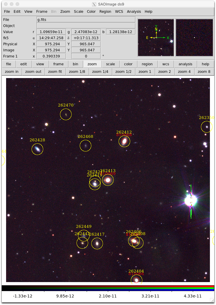

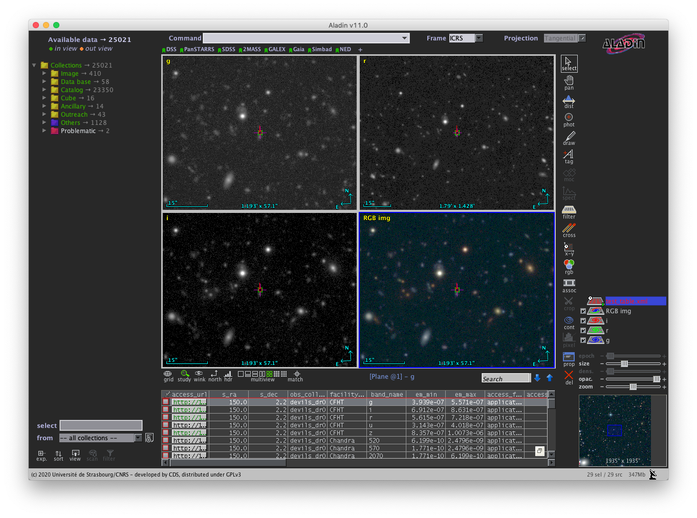
The result of running the above Python script using SIA to retrieve the images and SCS to generate the catalogues displayed as region files. With keyboard bindings and the cursor the user can load each object in the Single Object Viewer or query SIMBAD.

Access from Aladin

If you wish to access the SIA image cutouts from Aladin, you can follow these steps:

Generate and send a query to download your VOTABLE results to a file (e.g. test_table.xml).
Launch Aladin and choose the 'File->Load local file' menu item and select your VOTABLE file.
Once loaded, double click the filename layer at the lower right region of Aladin.
A table showing the VOTABLE rows and columns will appear at the bottom of the screen.
The access_url column contains clickable links to download each image.
You may select one of the multiview views just above the VOTABLE rows. This allows you to click several of the access_url links to populate each view with new image cutouts.

A screenshot below shows an example Aladin session as described above.

Aladin with SIA service generated VOTABLE and image cutouts. The RGB image was easily created by Aladin from the loaded image cutouts.

Access from TOPCAT with help from ds9

It is possible to access the SIA image cutouts from TOPCAT, which can send the image cutouts directly to the FITS viewer ds9 via SAMP.

Generate and send a query to download your VOTABLE results to a file (e.g. test_table.xml).
Launch TOPCAT and choose 'File->Load Table' and select your VOTABLE file.
Select the menu button for the Table Browser (Display table cell data).
Select the menu button with the Lightning Bolt on top of a table (Display actions invoked when rows are selected).
Check the 'Send FITS Image' item on the left hand side list.
Launch ds9. It may be necessary to choose the menu item 'File->SAMP->Connect' from ds9.
Select 'SAOImage ds9' from the Image Viewer drop down list. The Image Location should read 'access_url'
Now you can select rows in the Table Browser and they will automatically be sent to ds9.

A screenshot below shows an example TOPCAT session as described above.

Similarly, TOPCAT can also display the PNG image output from the SIA service. In this case no external viewer is required and instead of 'Send FITS Image', you can select 'Display image' which will send the PNG to TOPCAT's Basic Image Viewer.

TOPCAT and ds9 interoperability. The labels in the ds9 frames were added manually.

Documentation

Help Center

Simple Image Access Examples

Simple Image Access (SIA) service

Access from Python

Relatively quick access: Retrieving and parsing a VOTABLE

More advanced access: Using the pyvo module

Incorporating the pyds9 module

Using pyds9 to visualise multiple wavebands for a single object

Interacting with the Single Object Viewer (SOV)

Access from Aladin

Access from TOPCAT with help from ds9

data central

Data Access

Teams

User Support

About